On COVID-19 and Volatility Shocks in Energy Commodities

Dickson Pastory^*
*Correspondence: Dickson Pastory, Department of Accounting, College of Business Education, Dodoma, Tanzania, Tel: 255-713655380, Email:

Keywords

COVID-19 • Oil • Gas • SVAR • Economy

Introduction

The first case of unknown pneumonia that was later named Corona Virus (COVID-19) was reported in Wuhan, China in December, 2019 [1]. Since its first outbreak the disease has spread globally infecting over 185 million people with 4 million fatalities (WHO) [2]. The malignant virus has not only been a health crisis, rather it has fueled a global economic crisis whose magnitude resembles that of the great depression. COVID-19 has forced governments to impose containment measures such as lockdowns and travel restrictions that have adversely affected the global economy [3]. During 2020, the global economy shrunk by a staggtering 4% forcing 130 million people into extreme poverty [4]. The commodity market has suffered immensely as a result of economic downturn caused by COVID-19 [5]. COVID-19 containment measures have resulted into closure of businesses thus driving the commodities market on a downward spiral [6]. However this downward trend exhibited by commodities market has been unparallel among agricultural, metal and energy commodities with the latter expected to have long lasting effects. This is because the continuity of lockdowns, social distancing and workplace policies continues to take a toll on the energy market [7,8].

The global demand for energy commodities plunged by a staggering 4% in 2020 which is the steepest decline since World War II [9]. The global crude oil demand plummeted by 25% from January 2020 to April 2020 due to slowdown in economic activities especially transportation which accounts for two-third of global oil consumption [10]. The pandemic has also triggered a supply shock that ignited trade tensions between two major oil producers namely Saudi Arabia and Russia [11]. The natural gas market also fell by 4% in a similar time period which is astonishingly the largest drop ever recorded [12]. The disturbance in the global energy market amid COVID-19 has resulted into rising price volatility for the respective energy commodities. This price behavior has been experienced in past crises such as global financial crisis 2008 and SARS-COV outbreak [13]. In the case of crude oil, for the first time in history the price of West Texas Intermediate (WTI) plunged by 300% to only US$37 per barrel on 20^th April 2020 [14]. In the same period the Brent crude oil recorded the price of US$23 per barrel which is the lowest figure recorded in 17 years [15]. A similar downward spiral was experienced in the gas prices which recorded an average of US$2.11 per gallon in 2020, the lowest annual average in sixteen years period [12]. Rising volatility of energy prices has a significant impact on economic growth and prosperity around the world (The World Bank, 2020) [7]. Abrupt shocks in energy prices increase price uncertainty which affects businesses’ budgets for issues such as production costs leading to postponement of investments [4].

This article adds to existing knowledge on three folds. Firstly, it employs the novel Corona Panic Index (CPI) to assert whether panic created by media coverage of COVID-19 has an impact on global oil and gas price shocks. Negative news has a stronger power to influence and forecast volatility of commodity prices [16]. Unlike regional pandemics such as SARS-CoV and MERS-CoV, COVID-19 is a global catastrophe which has crippled the global economy [17]. So the impact of COVID-19 on price volatilities of major commodities is well examined on a global context [18]. Recent studies have focused their attention on studying price volatilities of energy commodities on country context [13,19]. However, the global context is more plausible as oil and gas are the engines of the global economy being vital inputs for most goods and services across the globe [20]. Their prices aggregately account for at least 50% of the general global commodity index [21].

The oil crisis in 1973 saw soaring oil prices that resulted into higher commodity prices thus triggering a global recession [22]. During the global financial crisis 2008, oil and gas prices slumped due to contraction in their demand triggering losses and staff layoffs in the energy sector as well as long run price overshoot [23,24]. Given profundity of oil and gas prices stability for the global economic prosperity, it is worth modeling the extent to which COVID-19 induced global panic affects oil and gas prices on the global scale. This examination is crucial for energy companies, investors, governments and other market agents as energy price volatility affects them altogether [25].

Secondly, the attention of current studies on COVID-19 and energy commodities has been mainly on oil [5,6,8,11]. A few studies such as have compared oil and gas volatilities during COVID-19 but on country context. Natural gas which is the second most traded energy commodity has been given little attention despite its growing enormity to the global economy. Natural gas accounts for at least 24% of the global energy consumption and its use gradually increases amid global plans to reduce coal consumption due to environmental concerns. Given increasing importance of natural gas to the global economy, modeling how the commodity’s price reacts to shocks caused by panic as a result of crises such COVID-19 is worth scholarly attention [26,27].

Thirdly, the study employs the SVAR model to assess the phenomenon at hand. SVAR allows simulating how past values of endogenous variable as well as dynamic shocks in exogenous variables affect the endogenous variable [28]. SVAR is more appropriate than VAR as the latter can only predict response endogenous variable based on its past values alone [29]. SVAR is employed to model how dynamic shocks created by COVID-19 global panic affect both oil and gas price volatilities. The rest of the paper is organized as follows literature review, discusses data and methods, results and conclusion.

Literate Review

Energy prices have shown reaction to past crises such as financial crises, pandemics, war and terrorist attacks. The tendency of energy prices to quickly and accurately change in response to relevant information is known as energy market efficiency [30]. This depiction is borrowed from the Efficient Market Hypothesis (EMH) by Fama [31], who advocates that in an efficient market, prices of financial assets at any point fully reflect all available information. However, if all relevant information is confined to past prices, then the market is considered to exhibit weak-form efficiency. Over the years empirical evidence such as [32-35] have shown that assets prices react to new information thus they can be forecasted.

Empirical studies have shed light on how energy prices volatility is affected by occurrence of major crises. Kumail, et al. [13], conducted a comparative assessment of oil price volatility during the global financial crisis of 2008, SARS-CoV and COVID-19. Using symmetric GARCH (1,1) and the asymmetric GJR-GARCH (1,1) they observed that oil prices behaved more volatile during COVID-19 due to the severity of the crisis. In another study by Ye, et al. [36] employed the Distributional Event Response Model (DERM) and observed significant rise in volatility of oil price during the U.S. invasion of Iraq in 2003 and the global financial crisis in 2008. Phan et al. investigated how oil prices react to terrorist attacks such as the London Bombings and World Trade Centre September 11 attacks. They showed that oil prices increase volatility due to terrorist attacks due to distortion in production and investment channels [37].

The current COVID-19 pandemic is no exception as it has brought unprecedented levels of uncertainties in the energy market (IEA, 2021) [9,11], observed that COVID-19 has adversely impacted the global energy commodities demand and supply. This increased uncertainty in the market which created significant price shocks in the West Texas Intermediate (WTI) as the pandemic continued running roughshod around the globe. These findings are supported by Shaikh [8] who discovered unprecedented levels of volatility in crude oil price in WTI amid COVID-19 outbreak in 2020. In a study by Łukaszewska, et al. [26] the oil and gas price volatilities of economic powerhouses namely USA and Japan were examined during the first wave of COVID-19 from January-June 2020. They used the Auto-Regressive Distributive Lag (ARDL) model and found out that oil prices in USA exhibited a significant negative over reaction while gas prices unexpectedly showed a positive trend. However both oil and gas prices in Japan were negatively affected with the difference in price reactions between the two countries explained by unparalleled COVID-19 developments. In another country level study examined the nexus between COVID-19 cases and deaths on Saudi Arabia’s oil prices by employing the ARDL model. Their findings reveal that the surging number of cases in the country resulted into growing uncertainty accelerating oil price volatility [19].

The review of literature has revealed that majority of energy prices volatility and crises studies are focused on the crude oil commodity. This can be explained by the fact that crude oil is the most traded commodity in the world (WTO, World Trade Organization 2020) [38]. Furthermore, it is accounts for 39% of the global energy consumption as it can be refined into other commodities used in transportation, heating and electricity generation. Despite its importance, price volatility of natural gas during crises has not been given much scholarly attention. Understanding behavior of all major energy during crisis like COVID-19 is crucial for designing of policies to counter adversity of increased price volatility. This is attributed to the fact that increased volatility of energy prices is likely to spill over to other commodities thus impacting consumption, production and investment decisions [39]. So the study will fill this gap by examining price shocks in oil and gas as a result of COVID-19 induced global panics on the global spectrum.

Methodology

Data

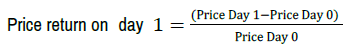
The data for the study ranges from 1st January 2020 to 30^th June 2021. The Corona Panic Index (CPI) statistics were retrieved from the website www. ravenpack.com. CPI measures the level of news chatter that makes reference to panic or hysteria and COVID-19. Values range between 0 and 100 where a value of 7.00 indicates that 7 percent of all news globally is talking about panic and COVID-19. The higher the index value, the more references to panic found in the media. The Brent crude oil price index is used for oil prices as it is among the renowned global benchmarks for the commodity’s price. The Brent crude oil price data were obtained from the website www.investing.com. The Henry Hub benchmark for natural gas prices was used for natural gas prices and its data were retrieved from www.yahoofinance.com. The daily price returns for crude oil and natural were used for analysis because the energy commodity prices are presented in different units of measurement. The returns were calculated using the following formula

COVID-19 Panic Index (CPI)

The detailed trend for CPI has been un-parallel in different months from January 2020 to June 2021. The panic started to build in February 2020 as COVID-19 started to spread across the world. However it was in March and April 2020 when the panic skyrocketed as explained by the fact it was during this period was when WHO firstly declared COVID-19 a public emergency with eventual declaration of the disease a pandemic (WHO, 2020) [40]. In the month of May 2020, CPI started to exhibit a downward trend however it was not smooth as daily panic showed sudden changes in panic. In June 2020, CPI started to smoothen with some visible sharp spikes in panic observed in October and November 2020. The month of December 2020 indicated sharp spike in panic as news of rising cases and deaths made headlines across the globe (WHO, 2020). However the panic dropped in January 2021 and exhibited a smooth trend to May 2021 when the panic started to spike again to June 2021. Figure 1 presents the trend of COVID-19 panic index.

Crude oil and natural gas

The trends for price returns for the above three named energy commodities are presented in Figure 2. Crude oil prices showed increasing volatility in the months from March-May 2020. This is the time period from which COVID-19 cases and deaths surged globally and the disease was declared a pandemic. From June 2020, prices exhibited a smooth trend with visible spikes far less significant like those from March-May 2020 appearing in the months of September 2020, November 2020 and March 2021. On the other hand, natural gas prices exhibit significant volatility with higher spikes both negative and negative being observed throughout the studied timeframe as opposed to crude oil. Higher magnitudes of volatility for natural gas were exhibited in June, August and September 2020.

Summary statistics

The summary statistics for the three variables are presented in Table 1. The results for CPI show that the mean for percentage of news covering COVID-19 issues that may cause panic and hysteria was 2.6%. The maximum coverage was 8.24% which may relate to early months in 2020 when the disease was declared a pandemic. The minimum coverage was 0% which relates to the early days of the pandemic in January 2020 when the virus had not yet gained global prominence. The mean natural gas price return was 0.038 with the maximum return of 0.2189 and a minimum of -0.104.

For the case of crude oil the mean price return was 0.0011 which is less than that of natural gas. However, the maximum return of 0.3155 is higher than that of natural gas and this relates to the months between March and May 2020 when oil prices were more volatile. The minimum crude oil price return was -0.244 which is steeper than the minimum natural gas return. These comparative results can be explained by the fact that crude oil exhibited far bigger negative and positive spikes than natural gas but only in the months between March-May 2020. For the rest of the months, natural gas price returns were more volatile than those of crude oil and this has been well elucidated in the discussions part.

Methods

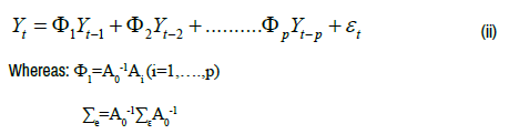
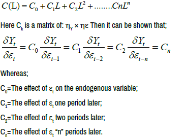
The SVAR model is utilized to examine the phenomenon at hand. SVAR is a multivariate linear representation of a vector of endogenous variables based on its own lags as well as other exogenous variables as a trend or a constant [28]. Unlike reduced form or recursive VAR models, SVAR permits setting of restrictions that allows examination of causal relationships between contemporaneous variables [29]. The residuals of the SVAR equations comprise of the primary structural economic shocks combinations with an assumption that they are orthogonal to each other [41]. The SVAR model is estimated as follows:

Whereas: Y=Endogenous variable; t=time period; ε_t=error term at time t.

This model operates on the following assumptions

• Any serial correlation within the exogenous variables is reflected in the lag polynomial C (L).

• C (L) is square and the general requirement for invertibility is that the fact that determinantal polynomial C(z) has all of its roots outside the unit circle.

To estimate SVAR, there are no restrictions for A0 to be diagonal and equation (i) above is treated as a dynamic simultaneous equations model. Though exogenous variables are not included in equation (i), they are treated similar to lagged values of endogenous variable “Y” for model identification and estimation objectives.

Equation (i) can be reduced into the following equation.

The relationships modelled by SVAR are then presented graphically in the Impulse Response Functions (IRFs). These graphs depict responses by an endogenous variable as a result of an impulse/shock from either an exogenous variable or lags of the same endogenous variable [42]. The representation of IRFs is as follows:

After IRFs estimations, the Forecast error variance decomposition (FEVD) is computed. The FEVD computes the percentage of error variability in forecasting endogenous variables Y₁ and Y₂ at time “t+n” based on information available at time “t” [43]. This error is a result of variability in the structural shocks ε1 and ε2 between times “t” and “t+n”. FEVD allows depiction of how profound an exogenous variable is in explaining shocks in endogenous variables.

Results

Pre-estimation diagnostics

Normality tests: The time series data for crude oil, natural gas and CPI were tested for normality which is a crucial prerequisite for multivariate time series analyses [44]. The Shapiro-Wilk test for normality was carried out and the results showed that the p values for all three variables are less than the 5% critical value. This is an indication that the time series data for these variables are normally distributed [45]. The results are presented in Table S1 in Appendix 1.

Unit root tests: The time series data for all the variables were tested for unit root. The Augmented Dickey-Fuller (ADF) test was carried out and the results for all three variables showed that their respective data are stationary. This is signified by the fact that their respective test statistic values were each greater than the 5% critical value [46]. The ADF results are presented in Table S2.

Lag order selection statistics: The selection of number of lags for the time series data pertaining to the three (3) variables was conducted as a prerequisite for conducting SVAR. Multivariate time series models such as SVAR operate on the assumption that each variable in the model is a linear function of its past lags as well as past lags of other variables [29]. Lag length estimation forms a critical part of SVAR modeling as it approximates the fixed maximum time for the past value of the same variable or other variables to take effect on a particular variable [47].

The Final Prediction Error (FPE), Akaike Information Criterion (AIC), Hannan Quinn Information Criteria (HQIC) and Schwartz Information Criteria (SBIC) were used as the criteria for lag length selection. The results portrayed that the maximum lag length to be eight (8) days for the AIC and FPE criteria while HQIC and SBIC both fixed the lag length to one (1) day. Since the number of observation is greater than 60, then SBIC and HQIC provide more correct estimation thus choosing the lag length of one day [48]. The results are presented in Table S3.

Causality diagnostics: The Granger causality test is employed to assess whether CPI is helpful in forecasting both crude oil and natural gas prices [49]. The p-values for both endogenous variables namely natural gas and crude oil were less than the 5% critical value. This is an indication that CPI is an important variable that can be put into use to forecast both crude oil and natural gas prices. The results for this particular test are presented in Tables S4 and S5 respectively.

Discussion

Structural vector auto regression estimation

The SVAR model is composed of crude oil and natural gas prices as the endogenous variables with CPI being the exogenous variable. The SVAR model is estimated by setting short-run restrictions in which some variables are prevented from reacting to some shocks on impact [50]. Short run restrictions are used instead of long run restrictions as the latter is not well equipped to properly recover the shocks [51]. The following short-run restrictions are imposed.

• CPI shocks cannot contemporaneously affect crude oil prices.

• CPI shocks cannot contemporaneously affect natural gas prices.

The iterative SVAR modeling is then carried out to model how CPI affects crude oil and natural gas prices. The results of this process are presented in the form of IRFs. The IRFs are developed for the exogenous variable (CPI) to model how its past values affect it. Then IRFs are developed for the impacts of CPI on each of the two (2) endogenous variables and then for the endogenous variables in relation to their past values.

Impulse response modelling results

Impulse response between lagged corona panic index and corona panic index: Figure 3 displays how shocks caused past values of CPI affect CPI across the time horizon extending from January 2020 to June 2021.

The results show that the initial shock to CPI occurred early within the first five months of 2020. This was around late January 2020 and presents the biggest shock to have occurred in the time frame to June 2021. The magnitude of this shock may be attributed to the immense panic in as in the period from January to March 2020 significant events occurred that may have gradually built panic. When the first cases were reported in China, the panic may have been minimal as the public in other parts of the world may have perceived the disease to remain regional similar to SARS-CoV and MERS-CoV

However in early January 2020, COVID-19 cases were being reported in other countries outside China which may have started creating fears around the globe. During January 2020 significant events occurred that may have caused the biggest shock in CPI in early February 2020. Firstly in late January 2020, the number of cases skyrocketed in the city of Wuhan in China and the city was put under quarantine [52]. Secondly, in 31st January 2020, WHO issued a global health emergency with infections skyrocketing in Japan, Taiwan, Vietnam, Germany and [40]. Accumulation of these events magnified by WHO’s declaration of the disease as a public emergency in late January 2020 sent massive fear and panic around the globe which explains the shock in the first period.

The initial shock started to wear down very slowly as the panic was still lingering as more bad news continued to dominate the global media. These include restriction of global air travel in February 2020, WHO’s declaration of COVID-19 a pandemic in March 2020, CDC announcement about death toll in USA surpassing 100,000 in May 2020 (WHO, 2020) [40]. However, there was also some promising news which may have helped to repel the effect of bad news on the public after the initial shock. These include the Food and Drugs Authority (FDA) authorization for the use of Hydroxychloroquine in March 2020. Also the reports by National Institutes of Health (NIH) that showed promise on the potential for remdesivir drug to treat COVID-19 [53].

A second spike in the global panic occurred in the middle of the second period ranging from May 2020 to October 2020. However the magnitude of this shock was not as large as the initial shock. It is likely that COVID-19 news from the previous periods coupled with significant events that occurred in July and early August 2020 may have triggered this shock. The WHO’s announcement that COVID-19 can possibly be airborne coupled with US reaching 3 million infections (WHO, 2020) thus causing tensions with WHO pertaining to its handling of the pandemic may have reignited the fears from the last 6 months.

Similar to the initial shock, the second shock also died down slowly into the third period ranging from November 2020 to March 2021. Another shock smaller than the previous shocks on global panic was observed at the end of period 3 in the month of March 2021. The lagged effect of news from the early months of 2021 combined with news of discovery of a highly contagious Delta mutant in Europe and USA in March 2021 [54], may have sparked panic around the globe pertaining to the potential for the pandemic to end. The third shock then slowly died down in a similar fashion to the previous ones into the fourth period from April to July 2021.

Impulse response between corona panic index on crude oil price: Figure 4 displays the response of crude oil price returns due to shocks originating from the CPI across the time horizon extending from January 2020 to June 2021.

The initial shock on crude oil price returns as a result of CPI occurred in the early months of the first period from January-February 2021. The initial shock sent crude oil returns to the negative and triggered a further sharp decline in returns that lasted for a period of at least a month between January and February 2020. This immense shock may be a result of widespread panic as a result of China’s decision to shut down its economy by imposing lockdowns and social distancing measures across major cities [52]. This decision led to a drop in global oil demand as China is the second biggest oil consumer thus forcing prices on a steep downward spiral. Failure by Russia and Saudi Arabia to agree on oil and production level adjustments to match demand may have also had a bearing on the magnitude of this shock [55,56]

The second smaller shock occurred in late February 2020 which resulted into a decrease in the rate of deterioration of crude oil returns. From February the returns kept on deteriorating but at a far smaller rate as opposed to the rate of drop observed in the initial shock. This may be a lagged effect of CPI which its initial magnitude had died down. The third shock occurred in late March which saw crude oil price returns starting to increase gradually until the second period from May-October 2020. This upward trend during this period can be likely associated with reduced global panic was reduced by the fact that countries during this timeframe started to emerge from lockdowns [57]. Furthermore the decision by OPEC and non OPEC members to curtail supply to match reduced demand helped to stabilize oil prices.

The fourth shock on crude oil price was observed in the second period around mid-June 2020 which for the first time since January 2020 saw the returns returning crossing 0 to the positive side. This is likely a lagged effect of reduced panic as countries started emerging from lockdowns in the previous month thus signifying recovery of oil demand. This was followed by a temporary sharp decline in returns to the negative which was then met with a fifth shock which occurred around August 2020 causing crude oil returns to start climbing again and return to the positive around September 2020. The returns maintained a smooth pattern in the positive side until a very small shock occurred around March 2021 which caused the returns to narrowly drop to the negative and quickly returned to the positive again. The visible positive trend from August 2020 is signified by the fact that in this month global oil prices rose to US$45 per barrel which is the highest amount since the beginning of lockdowns across the world [52]. As countries continued to emerge from lockdowns with the prospects for vaccines, the global panic was reduced prompting growth in demand [57]. There were no significant shocks in 2021 as the crude oil returns were mostly positive which is likely due to fading global panic as economies slowly recovered from COVID-19 catastrophe. This stability in crude oil prices was due to continued supply constraints by oil producers amid growth in demand [58].

Impulse response between corona panic indexes on natural gas price: Figure 5 displays the response of natural gas price returns due to shocks originating from the CPI across the time horizon extending from January 2020 to June 2021.

The initial shock for natural gas price returns occurred in the first period January-May 2020 which saw an initial drop in the commodity’s returns in January 2020. Despite this shock, returns remained positive and kept on climbing steadily until mid-February 2020 when the biggest shock occurred that abruptly drove natural gas returns to the negative side to April 2020. This may be likely due to elevated panic that occurred during February and March 2020.

During these months, WHO firstly declared COVID-19 a public emergency, however due to rising cases and deaths globally the disease was declared a pandemic in March 2020. This forced economies into lockdowns which adversely affected the global demand for natural gas as world’s largest importers cut demand. These include Japan, China and India that each experienced decline in natural gas demand amid lockdowns in the January- March 2020 [27]. Furthermore, during this demand deteriorated forcing prices downward due to mild temperatures during winter that reduced power consumption in heating [59]. The third shock in natural gas price also occurred in the April 2020 where the commodity’s price abruptly rose and maintained an upward trend to the second period. There was a small fourth shock in June 2020 which increased the steepness of the upward climb causing returns to finally cross to the positive side. The natural gas returns kept on climbing until August 2020. The upward price response to CPI may be a result of weakening panic as economies started to emerge from lockdowns. The steep upward response witnessed from June to August may likely be explained by rising demand during summer as more power is consumed for air conditioning appliances powered by gas-fired generators [60].

The fifth shock occurred in August 2020 as natural gas returns kept on climbing upwards but at a slower rate as opposed to the previous shock. This may be attributed to the fact that demand started to level off as summer season continued. The sixth shock was experienced in mid-September which saw a sharp decline in returns into November 2020 and slightly crossed into the negative. This was followed by the seventh shock whereby natural gas returns exhibited an upward trend back into the positive which is in the third period. The returns response to CPI Shocks in remained moderate as they exhibited a smooth upward then downward pattern on the positive side until period three which extends from February to June 2021. This smooth trend signifies weakening global panic as activities were returning to normal across the globe due to vaccination initiatives. Furthermore the natural gas production during this period was cut amid 2020-2021 winters which may likely have caused prices to rise (NGSA, 2020). The evidence of fading global panic on natural gas prices can be shown by the trends shown in the timeframes January-June 2020 and January-June 2021 in the impulse response function. The latter time frame was characterized by smooth response to panic shocks which mainly remained positive as opposed to the negative pattern observed in the same period in 2020 [59].

The Forecast Error Variance Decomposition (FEVD) Results

The FEVD results which help explain how important CPI is in explaining variations in crude oil and natural gas prices are presented in figure 6. The FEVD results indicate that for the case of natural gas, its own past prices were instrumental in forecasting future price for this commodity. The importance of CPI in explaining variations in natural gas price returns can be seen as low and its influence commenced in May 2020 and kept on rising gradually until June 2021. The percentage of shocks in natural gas prices explained by CPI was 12% which was the highest figure since January 2020. Crude oil prices had insignificant effect in causing shocks in natural gas prices.

However a different story can be told about crude oil. The magnitude of shocks in crude oil price as a result of CPI started at about 10% in January 2020. However, CPI’s influence on forecasting crude oil prices kept on growing to 40% in July 2020 and approximately the same influence was observed to June 2021. These results indicated that CPI had tremendous power to cause shocks in crude oil prices as opposed to natural gas prices. This can be explained by the fact that natural gas prices were already suffering in January 2020 even before the COVID-19 pandemic (NGSA, 2020). The unexpected mild temperatures during winter in 2019-2020 shrank natural gas demand causing prolonged deterioration in price in the early months of 2020. The outbreak of COVID-19 which further deteriorated demand amplified the existing problem. Another interesting fact is that natural gas prices had a percentage of bearing on shocks in crude oil prices. Shocks in crude oil caused by natural gas prices kept on growing until they reached approximately 10% in April 2020 and the same figure was maintained to June 2021.

Conclusion

This study examined whether panic and fear induced by COVID-19 global news coverage is associated with shocks in global prices of crude oil and natural gas. The findings provide evidence to show that panic caused by COVID-19 has caused major structural shocks in the two energy commodities. Furthermore the shocks were more severe and pronounced in the first five months of 2020 when the pandemic was spreading across the globe forcing countries into lockdowns to contain the disease resulting into the global economic slowdown. As a result natural gas and crude oil prices dropped due to the plunging demand for energy amid closure of factories, ports and restriction of air travel.

However the magnitude of shocks kept on decreasing along the time frame to June 2021 as the gradually panic died down as the global economy kept on recovering. The reduced panic may also be explained by prospects to contain the virus as nations around the globe started vaccinations rollouts. More importantly, the findings show that global panic induced by COVID-19 is more pronounced in explaining structural shocks in crude oil as opposed to natural gas whose prices were already suffering amid warm temperatures during winter in 2019-2020.

• The findings provide important insights to those involved in the oil and gas supply chains on the importance of taking early initiatives to restrict supply to match drop in demand during crisis. Failure to create this match results in volatile price movements which have widespread economic ramifications as oil and gas are among the most used inputs in different economic sectors. A drop in demand during crisis is usually expected in major crises such as the global financial crisis 2008. So when the supply is not restricted there will be oversupply in the global market forcing prices to plunge which may be beneficial to consumers in the short run. However in the long run oil and gas producers will cut supply which may cause a price overshoot with spill-over effects felt in other major economic sectors such as transportation and manufacturing. So the study stresses a need for all parties involved in crude oil and natural gas supply chains to take swift and calculated actions to restrict supply in order to match changes in demand during crises. This will help to ensure price stability amid crises which is profound for the health of oil producers as well as the global economy at large.

References

1. Remuzzi, Andrea and Giuseppe Remuzzi. “COVID-19 and Italy: What Next?” Rev Econ Stud 72 (2020): 821-852.
2. World Health Organization. “WHO Coronavirus (COVID-19)” (2021).
3. Morgan, Anthony Kwame, Beatrice Aberinpoka Awafo and Theophilus Quartey. “The Effects of COVID-19 on Global Economic Output and Sustainability: Evidence From Around the World and Lessons for Redress.” Sustain Sci Prac Pol 171 (2021): 77-81.
4. United Nations Conference on Trade and Development. “COVID-19’s Economic Fallout Will Long Outlive the Health Crisis, Report Warns.” (2020).
5. Mensi, Walid, Ahmet Sensoy, Xuan Vinh Vo and Sang Hoon Kang. “Impact of COVID-19 Outbreak on Asymmetric Multifractality of Gold and Oil Prices.” Resour Pol 69 (2020): 101-129.
6. Salisu, Afees A, and Kingsley Obiora. “COVID-19 Pandemic and the Crude Oil Market Risk: Hedging Options with Non-Energy Financial Innovations.” Financial Innov 7 (2021): 34-43.
7. The World Bank. “Impact of COVID-19 on Commodity Markets Heaviest on Energy Prices; Lower Oil Demand Likely to Persist Beyond 2021.” (2020)
8. Shaikh, Imlak. “Impact of COVID-19 Pandemic on the Energy Markets”. Econ Change Restruct 1 (2021): 1-52.
9. International Energy Agency. “Global Energy Review 2021.” (2021).
10. International Energy Agency. “Oil Market Report-April 2020.” (2020a).
11. Bourghelle, David, Fredj Jawadi, and Philippe Rozin. “Oil Price Volatility in the Context of COVID-19.” Int Econ 167 (2021): 39-49.
12. International Energy Agency. “The COVID-19 Crisis Highlights LNG’s Key Role in Global Natural Gas Security.” (2020b).
13. Syed, Kumail Abbas Rizvi and Rania Itani. “Oil Market Volatility: Comparison of COVID-19 Crisis with the Sars Outbreak of 2002 and the Global Financial Crisis of 2008.” Econ Res-Ekonomska Istraživanja 1 (2021): 1-22.
14. Devpura, Neluka and Paresh Kumar Narayan. “Hourly Oil Price Volatility: The Role of COVID-19.” Energy Res Lett 1 (2020): 78-103.
15. Deloitte. “Understanding the Sector Impact of COVID-19 Oil and Gas.” (2020).
16. Narayan, Paresh Kumar. “Oil Price News and COVID-19-Is There Any Connection?” Energy Res Lett 1 (2020): 78-92.
17. Laing, Timothy. “The Economic Impact of the Corona Virus 2019 (Covid-2019): Implications for the Mining Industry.” Extr Ind Soc 7 (2019): 580-582.
18. Umar, Zaghum, Saqib Aziz and Dima Tawil. “The Impact of COVID-19 Induced Panic on the Return and Volatility of Precious Metals.” J Behav Exp Finance 31 (2021): 100-125.
19. Algamdi, Abdelmageed, Said Khalfa Mokhtar Brika, Adam Musa and Khalil Chergui. “COVID-19 Deaths Cases Impact on Oil Prices: Probable Scenarios on Saudi Arabia Economy”. Front Pub Health 9 (2021): 620-875.
20. Trench, Cheryl J and Thomas O. Miesner. “The Role of Energy Pipelines and Research in the United States.” Pipeline Res Coun Int 1 (2006): 1-23.
21. Bašta, Milan, and Peter Molnár. “Oil Market Volatility and Stock Market Volatility.” Finance Res Letters 26 (2018): 204-214.
22. Mitchell, Timothy. “The Resources of Economics.” J Cultural Economy 3 (2010): 189-204.
23. Joo, Kyohun, Jong HwanSuh, Daeyong Lee and Kwangwon Ahn. “Impact of the Global Financial Crisis on the Crude Oil Market.” Energy Strategy Reviews 30 (2020): 100-116.
24. “IEA Calls Oil and Natural Gas Outlook Very Uncertain as Economic Crisis Hits Markets.” International Energy Agency (2009).
25. IEA Calls Oil and Natural Gas Outlook Very Uncertain as Economic Crisis Hits Markets.” International Energy Agency (2009).
26. Charles, F Mason and Wilmot A Neil. “Jump Processes in Natural Gas Markets.” Energy Economics 46 (2014):  78-92.  
27. “World Energy Balances: Overview Complete Energy Balances for Over 180 Countries and Regions.” International Energy Agency (2020).
28. Lukaszewska, Honorata Nyga and Kentaka Aruga. “Energy Prices and COVID-Immunity: The Case of Crude Oil and Natural Gas Prices in the US and Japan.” Energies 13 (2020): 63-87.
29. World Energy Balances: Overview Complete Energy Balances for Over 180 Countries and Regions.” International Energy Agency (2020).
30. Christopher A, Sims and Tao Zha. “Does Monetary Policy Generate Recessions? Macroeconomic Dynamics.” Cambridge University Press 10 (2005): 231-272.
31. Alvarez-De-Toledo, Pablo, Adolfo Crespo Marquez, Fernando Nunez and Carlos Usabiaga. “Introducing VAR and SVAR Predictions in System Dynamics Models.” Int J Simulation Process Model 4 (2008): 78-89.
32. Thai-Ha, Le and Nguyen Canh Phuc. “Is Energy Security a Driver for Economic Growth? Evidence from a Global Sample.” Energy Policy 129 (2019): 436-451.
33. Fama, F Eugene. “Efficient Capital Markets: A Review of Theory and Empirical Work.”  J Finance 25 (1970):  383-417.
34. Marobhe, Mutaju Isaack. “Investors' Reactions to COVID-19 Related Announcements: Evidence from the Cargo Shipping Industry.”Review of Behavioral Finance (2021).
35. Aboura, Sofiane and Niklas Wagner. “Extreme Asymmetric Volatility: Stress and Aggregate Asset Prices.” J Int Financial Markets Inst Money 41 (2016):  47-59.
36. Rakshit, Bijoy and Yadawananda Neog. “Effects of the COVID-19 Pandemic on Stock Market Returns and Volatilities: Evidence from Selected Emerging Economies”.  Studies in Economics and Finance (2021).
37. Gurrib, Ikhlaas. “Early COVID-19 Policy Response on Healthcare Equity Prices.” Studies  Eco Fin (2021).
38.  “World Trade Statistical Review 2020.” World Trade Organization (2020).  
39. Ye, Shiyu, Berna Karali and Octavio Ramirez. “Event Study of Energy Price Volatility: An Application of Distributional Event Response Model.”  AG Econ Search 27 (2014): 1-12,
40.  “WHO Coronavirus (COVID-19) Dashboard.” World Health Organization, (2020).
41. Bach Phan, Dinh Hoang, Paresh Kumar Narayan and Qiang Gong. “Terrorist Attacks and Oil Prices: Hypothesis and Empirical Evidence.” Int Rev Financial Analysis 74 (2021): 101-129.
42. World Trade Statistical Review 2020.” World Trade Organization (2020).
43. Maslyuk-Escobedo, Svetlana, Rotaru Kristian and Dokumentov Alexander. “News Sentiment and Jumps in Energy Spot and Futures Markets.” Pacific Basin Finance J 45 (2017): 186-210.
44. WHO Coronavirus (COVID-19) Dashboard.” World Health Organization, (2020).
45. Luca, Gambetti.  “Structural Vector Autoregressive Models.” Oxford Research Encyclo Economics Finance (2021).
46. Helmut, Lütkepohl. “Impulse Response Function. In: Palgrave Macmillan (editions).” The New Palgrave Dictionary of Economics (2008).
47. Helmut, Lütkepohl. “Estimation of Structural Vector Autoregressive Models.”  Commun Stat Appl Methods 24 (2017): 421-441.
48. Tomas,z Górecki, Hörmann Siegfried, Horváth Lajos and Kokoszka Piotr. “Testing Normality of Functional Time Series.” J Time Ser Anal 39 (2018): 471-487.
49. Samuel, Sanford Shapiro and Martin B Wilk. “An Analysis of Variance Test for Normality (Complete Samples).” Biometrika 52 (1965):591-611.
50. David A, Dickey and Wayne A Fuller. “Distribution of the Estimators for Autoregressive Time Series with a Unit Root.” J Am Stat Assoc 74 (1979): 202-305
51. Omer, Ozcicek and McMillin W Douglas. “Lag Length Selection in Vector Autoregressive Models: Symmetric and Asymmetric Lags.” Appl Econ 31(2001): 92-105.
52. Venus Khim-Sen, Liew. “Which Lag Selection Criteria Should we Employ?” Econ Bull 3 (2004): 1-9.
53. Gebhard, Kirchgässner, Wolters Jurgen and Hassler Uwe. “Granger Causality: Introduction to Modern Time Series Analysis.” STBE (2013).
54. David, Altig, Lawerence J Christiano, Martin Eichenbaum and Linde Jesper. “Firm-Specific Capital, Nominal Rigidities and the Business Cycle.” Rev Econ Dyn  14 (2011): 225-247.
55. Christopher J, Erceg, Guerrieri Luca and Gust Christopher. “Can Long-Run Restrictions Identify Technology Shocks?” J Eur Econ Assoc 3 (2005): 1237-1278.
56. Graham-Harrison, Emma, and Lily Kuo. “China's Corona Virus Lockdown Strategy: Brutal but Effective.” The Guardian (2020).
57. AJMC Staff. “A Timeline of COVID-19 Developments in 2020.” Am J Manag Care (2021).
58. Reuters, Fact Check. “Fact Check-Delta variant did not come from the COVID-19 Vaccine.” (2021).
59. “Global Energy Review 2020c-The Impacts of the COVID-19 Crisis on Global Energy Demand and CO2 Emissions.” IEA (2020d).
60. Akshay Kumar, Singh. “The “Oil War” of 2020 between Saudi Arabia and Russia.” IJAA 33 (2020):  24-42.