Research Article - (2025) Volume 14, Issue 1
Received: 17-Jan-2020, Manuscript No. JEES-23-6472;
Editor assigned: 22-Jan-2020, Pre QC No. P-6472;
Reviewed: 05-Feb-2020, QC No. Q-6472;
Revised: 06-Feb-2025, Manuscript No. R-6472;
Published:
14-Feb-2025
, DOI: 10.37421/2332-0796.2023.12.46
, QI Number: JEES-23-6472
Citation: Zerigui, Amel, Louis A Dessaint, Innocent Kamwa and Wassil Alaouni. "Dual-Kriging for Transient Stability Constrained Optima Power Flow by Using Detailed Machine Model." J Electr Electron Syst 14 (2025): 46.
Copyright: © 2025 Zerigui A, et al. This is an open-access article distributed under the terms of the creative commons attribution license which permits unrestricted use, distribution and reproduction in any medium, provided the original author and source are credited.
Transient Stability Constrained Optimal Power Flow (TSCOPF) is an important tool for power system planning and operation. It is a big challenge in the field of power systems because of its high complexity and extensive computation effort involved in its solution. This paper presents a new approach to compute the transient stability constraint formulated by the Critical Clearing Time (CCT) in TSC-OPF. CCT has been determined by Dual-Kriging, a space interpolation method which has primarily been used in natural resources evaluation. Given the huge dimensionality of the problem, Pareto analysis is firstly used to reduce the number of input variables in an initial database to those which are significant to compute CCT. With the reduced variables, a new database has been constructed using a design of experiment to obtain a reduced number of observed points. As a result of this approach, the sets of dynamic and transient stability constraints to be considered in the optimization process are reduced to one single stability constraint with only a few variables. Finally, the size of the resulting optimization problem is almost similar to that of a conventional OPF. In the new approach, there is no limitation for the machine model. The effectiveness of the proposed method is tested on the New England 10-machine 39-bus system by using detailed model and the larger power system 50-machine 145-bus power system.
Optimal power flow • Critical clearing time • Hurdle negative binomial • Count models
Modern power systems have grown in size and complexity because of increasing electricity demand and larger power transmissions over longer distances. However, it is essential that security and reliability be ensured in power system operation. The main condition for reliable operation of such systems is to maintain synchronous generators running in parallel with sufficient capacity to meet the load demand at any time. A secured power system is able to survive large disturbances without interruption of customer service. Therefore, for proper planning and operation, after a disturbance occurs, the system survives the ensuing transient and moves into an acceptable equilibrium point where all components are operating within established limits.
Several methods have been investigated to determine the instability caused by a severe disturbance or a series of disturbances. These methods fall in two main categories. Conventionally, time domain simulation is used to solve the set of nonlinear equations describing the system variables. Time domain simulation is an accurate method but it eventually suffers from extensive computation effort for complex and large power systems. Direct methods are an alternative to time domain simulation.
Although transient energy based methods such as Extended Equal Area Criterion method (EEAC) provide techniques to assess the transient stability without solving the complex differential-algebraic equations set, transient energy based methods require many computations to determine the transient stability index and are difficult to implement in practice.
Optimal Power Flow (OPF) has always been an active research topic because of its practical value for power system economic operation. By including a transient stability constraint, the OPF is transformed into a Transient Stability Constrained OPF (TSC-OPF) which ensures that the optimal operating point is secured against a predefined contingency. A number of methods have been proposed to include the transient stability constraints in an OPF. Used a function transformation technique to convert the original TSC-OPF into an optimization problem via a constraint transcription. have converted dynamic equations to numerically equivalent algebraic equations and then integrated them into the standard OPF formulation. In order to decrease the size of the problem, a reduced admittance matrix was considered into reduce the number of constraints [1]. Instead of considering a transient stability constraint into the TSC-OPF general formulation, considered the re-dispatching of generation by modifying the critical machines power output limits into the conventional OPF analysis to obtain a near-optimal solution. Reduced the transient stability constraints to a single transient stability constraint by using a single machine equivalent method with a one-machine infinite-bus reference trajectory simulation up to the time to instability. Excluded the dynamic constraints from the optimization formulation by using an independent dynamic simulation. The same authors also proposed an approach based on dynamic reduction method where the single transient stability constraint is obtained by simulating the reduced system instead of the full system.
Modern heuristic optimization methods such as Evolutionary Algorithm (EA) have been applied to TSC-OPF. Cai et al., used the differential evolution algorithm for TSC-OPF. Yan, et al., combined a classical deterministic programming technique and an evolutionary algorithm for solving the problem of TSC-OPF. EA based methods have strong global searching capability; however, their computation burden can be very high.
Genc et al., used decision trees to determine security regions and their boundaries to predict the status of the system and to provide guidelines to take the necessary preventive or corrective control actions against transient instabilities. They estimate the dynamic secure boundaries by a linear combination of decision tree rules, and then the result is used for generation rescheduling and load shedding. This method was tested on the Entergy system and the secure operating point is found after the first iteration. Decision tree learning is one of the most successful techniques for supervised classification learning. A decision tree is fast, simple to understand and interpret. However, decision-tree learners can generate overcomplex trees that do not generalize well from the training data; pruning is needed to avoid this problem, so the explicit rules can be acquired for use. Besides, there are concepts that are hard to learn because decision trees do not express them easily, such as XOR or multiplexer problems. In such cases, the decision tree becomes very large. In addition, the decision tree tends to be sensitive to small changes of the data.
Under a similar knowledge extraction and utilization framework, Xu et al., developed a method for preventive dynamic security control for power systems. They extract patterns from a feature space characterized by critical generators. The patterns are a set of nonoverlapped hyper rectangles representing the dynamic secure/ insecure regions of the power system. The preventive control involves driving the insecure OP into the secure region. In practice, this method can be achieved by formulating the secure patterns as generation output constraints into an OPF model [2]. This method is tested on the New England 10 machine 39 bus considering both single and multi-contingency conditions.
To reduce the computation time burden, we propose a new methodology to solve the TSC-OPF problem. The main idea of this paper consists of developing a new method to estimate CCT by Dual-Kriging and subsequently include this stability index in a single transient stability constraint of the TSC-OPF formulation. The specific steps of the approach proposed in this paper are as follows:
• An initial database is treated by Pareto analysis. This method
finds the parameters which contribute significantly in computing
CCT. By using Pareto analysis, 80% of variables are reduced.
Pareto analysis provides only significant variables which are less
than 20% of the entire variables. This approach is tested on two
power systems which are 10 machines-39 bus and 50
machines-145 bus.
• A new database is designed by varying the significant variables
yielded by Pareto analysis and fixing the non-significant
parameters in the solution of the optimal power flow. The design
of experiment (Taguchi approach) is used to create the new
database; the objective of this step is to reduce the number of
operating points of the new database.
• After computing the CCT of operation points of the new database
by time domain simulation, Dual-Kriging is used to establish an
analytic derivable function that estimates the CCT.
• The first and second derivatives of the estimated CCT are
computed and the single transient stability constraint and its
derivatives are included in the OPF formulation.
It can be seen that the advantage of our statistical approach is that it supplies analytical expressions for the CCT as well as for its first and second derivatives; this reduces significantly the computation time of the TSC-OPF. Moreover, the analytical expression of the CCT is obtained very efficiently thanks to the Pareto analysis that reduces the number of independent variables and to the Taguchi method that reduces the size of the database. Even though CCT and a detailed machine model are employed in this study and only the single contingency is considered, the proposed methodology can be generalized to any transient stability index. Moreover, TSC-OPF with multiple contingencies can also be handled without any complexity by simply adding an additional transient stability constraint for each contingency.
Transient stability constrained optimal power flow
A TSC-OPF is basically defined as a nonlinear constrained optimization problem which consists of an objective function f(pg) and a set of equality and inequality constraints. The following optimization problem represents a TSC-OPF formulation.

Where ai, bi and ci are the generation cost coefficients of the ith generator, Pgi and Qgi are the active and reactive output of the ith generator, Pdi and Qdi are the load in the ith bus, Vi and Vj are the voltage magnitude of the ith and jth bus respectively. Gij and Bijare conductance and susceptance between the ith and jth bus, respectively. By adding the transient stability constraints, the power system is represented by a set of Differential Algebraic Equation (DAEs) as:
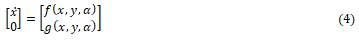
Where x is a vector of dynamic state variables such as generators angles, y is a vector of algebraic variables, and α is control parameters such as active power output of generators. The DAEs can be solved by implicit trapezoidal integration in time domain simulation. In most papers, the transient stability index is expressed by the angle threshold. In this paper, the CCT has been considered as a transient stability index [3]. The proposed method adopts Dual- Kriging to model the CCT as analytic function which is continuous and differentiable, as is explained. The transient stability constraint is therefore formulated as an equality constraint in TSC-OPF as:

Where tf represents the fault clearing time. The CCT function depends on the control variables which are generator bus voltage magnitude Vgi and generator bus active power Pgi. During the optimization procedure, since Vgi and Pgi are the control variables, the CCT changes accordingly to satisfy. It is important to point out that in the proposed method, the TSC-OPF formulation is defined and consequently DAEs solution is not required.
Detailed generator model (Two axis model)
In this paper a two-axis model of a generator with the IEEE-type I exciter are adopted.
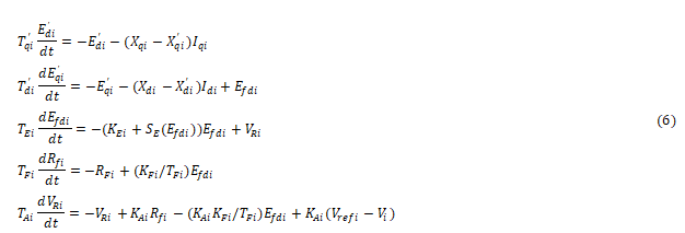
Where Td and Tq are the open circuit d-and q-axis transient time constants. Edi, Eqi represent the d-and q-axis components of the generator internal voltage [4]. Efdi, Rfi and VRi are the dynamic variables of the exciter. Idi, Iqi are d- and q-axis stator currents. Xdi, Xqi are the d- and q-axis transient reactances.
TEi, KEi, TFi, KFi, TAi, KAi are the exciter parameters. Vrefi is the reference input of the exciter, and Vi is the voltage amplitude of the bus i.
The stator algebraic equations for generator i are given by:
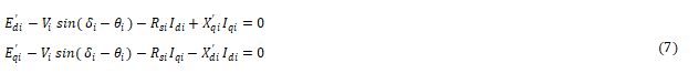
Where Rsi is the generator stator resistance. өiis the voltage angle of bus i.
Proposed method
Initial database: The database is a set of generated operating points (x) and the corresponding transient stability index i.e., the Critical Clearing Time (CCT). The generators’ voltage magnitude Vgi and the generators’ active power Pgi are taken as the input and the corresponding CCT as the output in this database. The resulting database is analyzed using Pareto analysis as explained below.
Pareto analysis for input dimension reduction: Identifying input variables that are critical for computing CCT by quantifying their risk is an important task. A power flow solution and dynamic parameters of the system are needed to compute CCT by using time domain simulation method [5]. Since the input parameters become numerous if the network is large, it is very important to identify the variables which influence the CCT quantitatively and qualitatively.
There are few published methods that quantify the variables importance for CCT calculation. Principal component analysis was used into reduce the input variables to neural networks for CCT estimation. Two sensitivity based methods have been used to select the input variables for training neural networks in. The first method is the sensitivity analysis which ranks the input variables by importance but does not quantify how much these input variables are important. Principal component analysis has been used as second method to reduce the components obtained by the first method. Besides, the correlation analysis method and the principal component analysis have been used in to reduce the input parameters. Neural networks have been used as a regression method in all the above approaches.
RELIEF algorithm is used in for selecting the critical operating variables. It is a statistical learning technique consisting of a feature weighting selection method. In this algorithm, the features are selected via a distance-based feature estimation process. The main concept of this algorithm is to compute a ranking score for every feature indicating how well this feature separates neighboring samples. Kira and Rendell proved that ranking score becomes large for relevant features and small for irrelevant ones. The key idea of RELIEF algorithm is to estimate the quality of features according to how well their values distinguish among instances of different classes that are near each other. The algorithm analyses each feature based on a selected subset of samples. For each randomly selected sample X from a training data set, it searches for its two nearest neighbors: one from the same class, called nearest hit H, and the other one from a different class, called nearest M. The original RELIEF algorithm is limited to only two-class problem. For this, Kononenko extended RELIEF algorithm to deal with noisy, incomplete and multi-class data sets, and also RELIEF algorithm is extended to K-nearest neighbors search. The selection of the nearest neighbors is an important factor in RELIEF. Redundant and noisy attributes may affect the selection of nearest neighbors and therefore the estimation of probabilities on noisy data becomes unreliable. Kononenko increased the reliability of probability approximation by extending RELIEF to search for K-nearest hits/misses instead of only one near hit/miss. Due to its effectiveness, simplicity and efficiency, RELIEF algorithm is considered one of the most successful methods. Since the RELIEF algorithm is an iterative calculation process of feature’s weight, the calculation for a system with large number of features might take much computing time.
Single Machine Equivalent (SIME) method is based on finding the single-machine equivalent of the multi-machine system. SIME technique relies on the observation that the loss of synchronism in a power system occurs due to irrevocable separation of machines into two groups: Critical Machines (CMs) and Non-Critical Machines (NMs) [6]. Based on Time Domain (TD) simulations, SIME uses the physical parameters and time-varying data of CMs and NMs to generate an equivalent machine for each group. These two machines are used to construct an OMIB (One Machine Infinite Bus) equivalent. SIME method provides accurate and reliable assessment of system information following a disturbance. SIME is a very convenient method in the determination of transient stability because it computes the time to instability (tu) or the time of return (tr) at which one can deduce formally the transient stability for a given contingency. However, SIME uses the results of a time domain simulation. Therefore, the accuracy of the SIME results is the same as for the simulation and the computation burden of SIME is slightly higher than for the simulation itself.
The proposed method in this paper is Pareto analysis. Pareto analysis is a statistical method that ranks data in decreasing order from the highest to the lowest frequency of in luence. It is based on 80/20 rule which means that in anything a few (20 percent) are vital and many (80 percent) are trivial or 20% of the input creates 80% of the result. In reality, Pareto does not demand that the 80/20 ratio applies to every situation. Often the optimal ratio is obtained by the smallest proportion that will produce the greatest improvement. The reasons that 80/20 has become the standard ratio associated with the effect are: the 80/20 correlation was the irst to be discovered and published and since its discovery, the 80/20 ratio has always been used as the name of the Pareto theory [7]. The Pareto principle is helpful in bringing swift and easy clarity to complex situations and problems. The Pareto principle is an extremely useful model or theory that can be applied to complex applications such as management, demographics, social study, all type of distribution analysis, evaluation and inancial planning and also electrical engineering such as wireless communication network [24], integrated circuit fabrication, analyzing controller design methodologies etc. In this paper, statgraphics software was used to perform the Pareto analysis.
Considering an initial database of uniformly distributed operating points for twenty variables (Vg1,…,Vg10), Pgi,…,Pg1) and based on their corresponding CCT, Pareto analysis ranks the most statistically signi icant variables as shown in Figure 1 as a standardized Pareto chart. The length of each bar is proportional to the value of a t-statistic calculated for the corresponding effect of the variable on CCT. The vertical line on the Pareto chart is the threshold value which indicates statistical signi icance level of 5% of the variable on CCT at 95% con idence level. From Figure 1, it is observed that Pareto analysis identi ies three parameters (Vg8, Vg9, Pg9) that are statistically significant while the other seventeen parameters are not important in this system.

Figure 1. Standardized Pareto chart.
Design of experiment for reduced database size
After identifying the input variables that contribute in computing CCT, a new database has been constructed. By using the Design of Experiment (DoE), the space of design can be covered with a few points. Thus, Taguchi approach has been adopted in this paper. For example, consider the above three variables (Vg8,Vg9,Pg9) which are significant in computing CCT and we want to construct a database with 7 levels (6 equal intervals) for each variable xi having minimum ximin and maximum ximax where ximinimax is the range (A range of ± 10% of OPF operating point was chosen for each variable). We would normally obtain a database with 73=343 operating points, but Taguchi approach reduces this database to 49 operating points where only weighted points are taken [8]. The corresponding CCT for each operating point is then computed using time domain simulation. With this reduced database, Dual-Kriging is used to model CCT as an analytic function as explained below.
Dual-Kriging estimation
Kriging is a statistical technique which was irst proposed by Krige for natural resources evaluation. The method was mathematically established by Matheron and was inally developed as Dual-Kriging by Trochu. Kriging as presented in geostatistics is simply the best linear unbiased estimator of a random function. It integrates several interpolation techniques such as Bezier, Splines and piecewise interpolation. The least squares method can be found as a limit case of Kriging. Dual-Kriging offers many advantages:
• Kriging function can take several forms such as linear,
polynomial, trigonometric and quadratic.
• Dual-Kriging method presents a common mathematical form for
representing both standard analytical shapes and free form
curves and surfaces.
• Fewer data points are needed to define curves and surfaces.
• No weights, control points or knots are used.
• The interpolation passes throughout the data points.
• The model can be updated.
Similarly, Dual-Kriging also offers several advantages for transient stability index estimation summarized as follows:
• The data base needed to find transient stability index requires
few operating points
• The transient stability boundary function is continuous and
differentiable. This is a very useful property since it allows
describing the transient stability constraint as an analytic
function in TSC-OPF.
• Transient stability index function is formed as a nonlinear
function of the power system variables.
• It has high accuracy and computational efficiency [9].
Basically, Kriging is an approach that allows the construction of an estimate function f(x)

Where n is the number of operating points. In Kriging, the unknown function f(x) is decomposed into the average behavior a(x) and a fluctuation (error term) b(x) then f(x) becomes as follows:

Where a(x) called the drift can be represented by a constant, polynomial, or even trigonometric function.
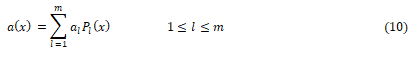
Where Pl(x)a basis function and are its coefficients.
The fluctuation b(x) is adjusted in Kriging. It depends on the observation points, and is weighed by correction function gj(x)the coefficients as follows:
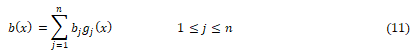
The correction weights associated to the data points depend only on Euclidean distance |x-xj| and then gj(x) becomes as follows.

Where K(h) is a function of the Euclidian distance h between two measurement points. In this paper, the Dual Kriging method is used to build an interpolation function f from a set of computer simulations.
If we assume that the vector of the design variables is (x,y,z), the function f(x,y,z) is the interpolation function. In this paper, the drift is chosen as a constant:
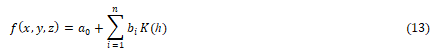
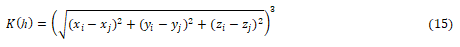
K(h) can take several forms, among them a cubic form as:

The cubic form is used in this paper; K(h) is the connection between two measurement points (xi,yi,zi) and (xj,yj,zj). Therefore K(h) is (13).
In matrix form (11) becomes (14)

Where H, A, B and F are matrices and vectors with the following forms:
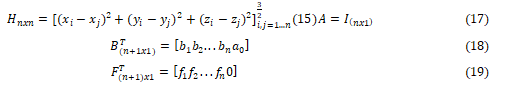
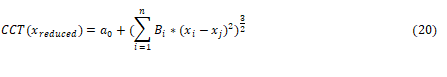
Where n is the observed points number in a database and F is the computer simulation solutions. In transient stability constraints fi represents CCTi, after solving (14) and obtaining the vector B which contains the coefficients of the drift and the correction term [10]. The CCT function can be expressed as given in the following:
Solution procedure
The estimated CCT presented by (19) will be used as an equality constraint, and then the problem of TSC-OPF presented by (1) to (4) will be similar to that of OPF. Therefore the TSC-OPF is basically a nonlinear optimization problem; the standard optimization solution methods must be modified to be able to solve this problem [11]. In this approach, an Interior Point method is used to solve the proposed optimization problem which first transforms all inequality constraints (3) into equalities by adding nonnegative slack vector si and then incorporate them into logarithmic barrier terms as follows:
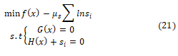
Where μS ϵ R is the barrier parameter to solve the equality constrained problem and si>0. Lagrangian function is defined.
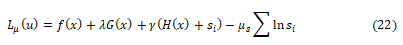
Where λ and γ are Lagrange multipliers, and u=[xT, sT, λT, γT]. A local minimum is expressed in terms of a stationary point Lμ(u), which must satisfy the Karuch-Kuhn-Tucker (KKT) optimality firstorder necessary conditions ∇μ L μ(u)=0. This problem is nonlinear, its solution is usually approximated by Newton’s method; whereby the Hessian is required in the algorithm. The computation of the Hessian ∇x2Lμ(u) requires the evaluation of the objective function Hessian ∇x2f(x) and the Hessians of equality and inequality constraints ∇x2G(x) and ∇x2H(x), since
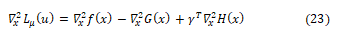
Where ∇x2G(x) is the Hessian of the equality constraints which include the Hessian of power flow equality constraints and the Hessian of transient stability constraints as presented below:

To obtain a solution to this, the exact computing ∇x2 CCT(x) is needed. The first and second derivatives are presented by (24) and (25) respectively.
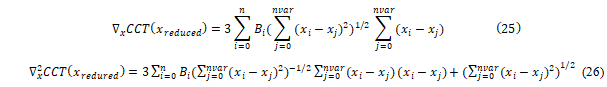
Where nvar is the number of variables. Equation (25) is needed to compute the Lagrangian function in (22) and (26) is required for computing the Hessian in (23).
Implementation of TSC-OPF
The computational procedure used to solve the proposed TSCOPF using interior point technique is shown in Figure 2 where the first and the second derivatives of CCT are calculated at every iteration [12].

Figure 2. TSC-OPF solution procedure.
This procedure can be summarized as follows:
• Run a conventional OPF to obtain an initial operating point.
• Start optimization i=1.
• Compute the static equality and inequality constraints by using
(2) and (3) as well as their derivatives.
• Compute CCT using (20) and its first and second derivatives by
using (25) and (26) respectively.
• Include the CCT-based stability constraint in (5) with the other
equality constraints in (2) as well as its derivatives.
• The KKT optimality conditions are formulated and solved using
interior point method, and the barrier parameter μs is updated.
• If the barrier parameter, the objective function and the
optimization variables converge within the given tolerance, then
the process stops, otherwise it is repeated from step 3.
Numerical examples
In order to illustrate numerically the practical application potential of the proposed method to control the transient stability, two power systems are tested: The New England 10-machine 39-bus system and the 50-machine 145-bus system. The two axis generator model is considered in New England system and the classical model is used in 50-machine 145-bus system. In the case studies, the conventional OPF has been solved using MATPOWER 4.0b4. A mixed 0.01 and 0.001 s integration time step has been considered in dynamic simulation to prepare the databases. The dynamic simulation program is written in Matlab. The initial database for each case, which is used in the study of sensitivity, contains 1500 uniformly distributed points around ± 10% of OPF operating point. The second database is constructed by Taguchi approach to obtain 49 points and is employed in the estimation of CCT function, except case A, a database of 25 operating points is used. All tests were performed on a PC with AMD PhenomTM II X4 B93, 2.79 GHz CPU and 4 GB RAM, with MATLAB 7.9.0 (R2009).
New England 10-machine 39-bus system: The data of the New- England system were taken from and fuel cost parameters from. The initial operating point computed by OPF provides the optimum power dispatch presented in Table 1. Three contingencies listed in Table 2 are considered, and their CCT on the initial Operating Point (OP) are also computed. In this section, three TSC-OPF calculations with single contingency are conducted as listed in Table 2 which are A, B and C [13]. The time domain simulation time is set up to 5 s and the mixed integration step is 0.01 and 0.001 s. The reduced parameters for each contingency are presented in Table 3. It is important to note that the reduced parameters pertain to buses which are close to the fault.
| Node | Generator cost ($/h) |
Generation (MW) |
Total cost ($/h) |
|---|---|---|---|
| 31 | 0.0193P2+6.9P | 566.44 | 60915.01 |
| 32 | 0.0111P2+3.7P | 642.37 | |
| 33 | 0.0104P2+2.8P | 629.86 | |
| 34 | 0.0088P2+4.7P | 508.1 | |
| 35 | 0.0128P2+2.8P | 650.59 | |
| 36 | 0.0094P2+3.7P | 558.51 | |
| 37 | 0.0099P2+4.8P | 534.99 | |
| 38 | 0.0113P2+3.6P | 830.28 | |
| 39 | 0.0071P2+3.7P | 976.17 |
Table 1. Initial operating point of New England system.
| Contingency | Fault location | Tripped line | Fault duration | CCT (s) (Initial OP) Dual-Kriging | CCT (s) (Initial OP) TDS |
|---|---|---|---|---|---|
| A | Bus 29 | 29-26 | 0.1 | 0.0913 | 0.091 |
| B | Bus 21 | 21-22 | 0.16 | 0.1399 | 0.14 |
| C | Bus 4 | 45050 | 0.25 | 0.229 | 0.229 |
Table 2. Contingency list for New England system.
| Contingency | Initial Input parameters | Reduced parameters | Vital parameters | Trivial parameters |
|---|---|---|---|---|
| A | 20 Variables (Pgi and Vgi) | Vg8, Vg9, Pg9 | 0.15 | 0.85 |
| B | 20 Variables (Pgi and Vgi) | Vg6, Vg7, Pg6, Pg7 | 0.2 | 0.8 |
| C | 20 Variables (Pgi and Vgi) | Vg2, Vg3, Pg2, Pg3, Pg10 | 0.25 | 0.75 |
Table 3. Input features for New England system using Pareto analysis.
The performances of the Dual-Kriging are evaluated using Root Square Mean Error (RMSE), Standard Deviation (SD) and mean absolute error between Dual-Kriging output and simulated (target) values as shown in Table 4.
| Power system | Contingency | RMSE (s) | SD (s) | Mean absolute error (s) |
|---|---|---|---|---|
| New England | A | 0.0102 | 0.0061 | 0.0082 |
| New England | B | 0.0143 | 0.0094 | 0.0108 |
| New England | C | 0.0125 | 0.0068 | 0.0105 |
Table 4. Performance of the estimated CCT for new England.
For the given contingencies, one published solution is collected from for benchmarking with the results obtained from the proposed method by using detailed machine model as is shown in Table 5 [14].
| Node | A | B | C |
|---|---|---|---|
| 30 | 243.013 | 245.494 | 239.044 |
| 31 | 568.027 | 572.374 | 545.123 |
| 32 | 644.044 | 648.684 | 604.843 |
| 33 | 631.802 | 637.635 | 625.265 |
| 34 | 509.434 | 513.421 | 504.963 |
| 35 | 652.472 | 619.763 | 646.134 |
| 36 | 560.277 | 536.633 | 554.348 |
| 37 | 536.872 | 540.457 | 531.467 |
| 38 | 814.059 | 838.644 | 824.719 |
| 39 | 978.882 | 986.106 | 1062.01 |
| CCT (s) Dual-Kriging | 0.1 | 0.16 | 0.25 |
| CCT (s) TDS | 0.1 | 0.16 | 0.25 |
| CPU Time (s) | 1.21 | 1.18 | 1.16 |
| Cost ($/h) | 60917.5 | 60933 | 60987 |
| ΔCost ($/h) | 2.48 | 17.96 | 71.97 |
| ΔCost ($/h) literature | Never reported | Never reported | 833.65 |
Table 5. TSC-OPF power dispatch for New England system.
Figure 3 illustrates the stable machine relative angle (degree) after the proposed TSC-OPF. The new operating point is found after the first iteration, the execution time of TSC-OPF is very low as shown in Table 5. Figure 4 shows the generator output change (MW) with respect to the initial operating point which is the OPF. In this case, the machine number 9 is considered as the leading machine in the system. Figure 3 shows the stable machine relative angle (degree) after the proposed TSC-OPF. The new operating point is found after the third iteration; also, the execution time of TSC-OPF is very low. Figure 4 illustrates the generator output change (MW) with respect to the initial operating point which is the OPF. In this case, the machines number 6 and 7 are considered as the principal machines. Figure 5 shows the stable machine relative angle (degree) after the proposed TSC-OPF. The new operating point is found after the second iteration. Same as the other cases, the execution time of TSC-OPF is very low as shown in Table 6. Figure 8 shows the generator output change (MW) with respect to the initial operating point. In this case, the machines number 2, 3 and 10 are considered as the dominant machines (Figures 3-8).

Figure 3. Stable relative rotor angles for case A.

Figure 4. Generator output change (MW) with respect to the initial OP for case A.

Figure 5. Stable relative rotor angles for case B.

Figure 6. Generator output change (MW) with respect to the initial OP for case B.

Figure 7. Stable relative rotor angles for Case C.

Figure 8. Generator output change (MW) with respect to the initial OP for case C.
50-Machine 145-bus system
The efficiency of the proposed approach is also demonstrated on the 50-machine 145-bus system that consists of 50 generators, 145 buses, 60 loads, 453 transmission lines and 52 fixed tap transformers. The data of IEEE 50-machine system were found in the software package Power System Toolbox (PST) [15]. The machine classical model is used for this system. The objective function of this case is to minimize the total cost associated with generation rescheduling as:
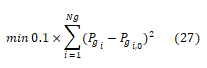
Where Pgi,0 is the initial active power of machine i. Pgi is the active power of the TSC-OPF. Ng is the total number of machines.
The test consists of stabilizing the system under a contingency defined by a three phase solid fault at bus 76 cleared by tripping the line connecting nodes 76 and 77. The initial CCT is 0.28 s, and we require that the CCT should be increased to 0.330 s. From Pareto analysis, we found that four parameters Vg6,Vg12,Pg6,Pg12 are very important for computing CCT. A database is prepared using these four parameters and Taguchi table yields a database with 49 operation points. After modeling the function with Dual-Kriging, we obtain an analytic function with only four parameters which represents the CCT of the 50-machine 145-bus power system for the given contingency. Time domain simulation is set to 5 s and integration step is 0.01 s.
Using the transient stability analytic function, the TSC-OPF is carried out by including this constraint into the optimal power flow constraints. The swing angles of the 50 machines after TSC-OPF procedure are plotted in Figure 7, which shows that the system is stable. Fig. 8 illustrates generator output changes with respect to the initial operation point. The TSC-OPF solution obtained with the proposed method is shown in. The operation point obtained by TSCOPF was validated by computing its CCT with time domain simulation (Table 6 and Figures 9, 10).
| Machine no. | Vg (pu) | Pg (MW) | Machine no. | Vg (pu) | Pg (MW) |
|---|---|---|---|---|---|
| 1 | 1.138 | 2001.409 | 2001.409 | 2001.409 | 2001.409 |
| 2 | 1.079 | 282.205 | 282.205 | 282.205 | 282.205 |
| 3 | 1.09 | 2505.546 | 2505.546 | 2505.546 | 2505.546 |
| 4 | 1.12 | 2725.303 | 2725.303 | 2725.303 | 2725.303 |
| 5 | 0.984 | 2638.604 | 2638.604 | 2638.604 | 2638.604 |
| 6 | 1.065 | 4233.39 | 4233.39 | 4233.39 | 4233.39 |
| 7 | 0.988 | 8969.102 | 8969.102 | 8969.102 | 8969.102 |
| 8 | 1.013 | 3008.473 | 3008.473 | 3008.473 | 3008.473 |
| 9 | 0.986 | 1008.297 | 1008.297 | 1008.297 | 1008.297 |
| 10 | 1.024 | 3009.319 | 3009.319 | 3009.319 | 3009.319 |
| 11 | 0.964 | 12982.589 | 12982.589 | 12982.589 | 12982.589 |
| 12 | 0.963 | 5951.559 | 5951.559 | 5951.559 | 5951.559 |
| 13 | 0.95 | 28316.528 | 28316.528 | 28316.528 | 28316.528 |
| 14 | 0.983 | 3106.516 | 3106.516 | 3106.516 | 3106.516 |
| 15 | 0.993 | 20642.492 | 20642.492 | 20642.492 | 20642.492 |
| 16 | 1.019 | 5999.248 | 5999.248 | 5999.248 | 5999.248 |
| 17 | 1.015 | 51967.39 | 51967.39 | 51967.39 | 51967.39 |
| 18 | 1.013 | 12081.395 | 12081.395 | 12081.395 | 12081.395 |
| 19 | 1.036 | 56850.928 | 56850.928 | 56850.928 | 56850.928 |
| 20 | 0.968 | 23139.395 | 23139.395 | 23139.395 | 23139.395 |
| 21 | 0.994 | 37927.574 | 37927.574 | 37927.574 | 37927.574 |
| 22 | 0.993 | 24465.214 | 24465.214 | 24465.214 | 24465.214 |
| 23 | 1.014 | 5267.974 | 5267.974 | 5267.974 | 5267.974 |
| 24 | 0.954 | 11412.962 | 11412.962 | 11412.962 | 11412.962 |
| 25 | 0.987 | 14135.157 | 14135.157 | 14135.157 | 14135.157 |
| CCT | 0.330 s | ||||
Table 6. TSC-OPF Power Dispatch for 50-machine 145-bus System.

Figure 9. Stable relative rotor angles for 50 machine-145 bus and contingency 76-77.

Figure 10. Generator output change (MW) with respect to the initial OP for 50 machine-145 bus and contingency 76-77.
This paper tests the detailed machine model by using a new approach which is based on statistical methods to realize TSC-OPF. This method allows the reduction of the computational burden of the extended OPF. Dual-Kriging, an accurate and fast method has been used to obtain the transient stability index (CCT) in functional form. Prior to applying the space interpolation method, Pareto analysis which is a sensitivity study was performed to reduce the number of variables to those which are only significant for computing CCT. Furthermore, based on a design of experiment, the Taguchi approach, the number of observed points in the database was reduced. The obtained CCT function was implemented in a single transient stability constraint to solve the TSC-OPF problem. The Interior Point Method (IPM) was used as optimization algorithm, because of its efficiency. However, this method requires the computation of the first and second derivatives of the constraints. The estimated function provided these two derivatives which facilitate the use of IPM, as consequence the TSC-OPF is solved in a short time.
The diversity of case studies that are discussed in the paper shows that the proposed TSC-OPF procedure is reliable and generally provides more economical results than other existing techniques.
Journal of Electrical & Electronic Systems received 733 citations as per Google Scholar report