Time Inconsistent Stochastic Differential Game: Theory and an Example in Insurance

Hong Mao¹, Krzysztof Ostaszewski^2*, Zhongkai Wen³ and Jin Wang^4
*Correspondence: Krzysztof Ostaszewski, Distinguished Professor of Mathematics and Actuarial Program Director, Illinois State University Normal, Illinois, USA, Tel: + 13092871711, Email:

Keywords

Stochastic differential game • Time-varying correlation • Extended HJBI equation • Equally weighted investment strategy • Investment and reinsurance

Introduction

The optimal-decision problem in investment and reinsurance has attracted many attentions from academia and industry. Most literatures use time-consistent dynamic programming, establish, and solve Hamilton–Jacobi– Bellman (HJB) equations to obtain optimal solutions. Browne studied optimal investment decisions for a firm with an uncontrollable stochastic cash flow. Applied Cramer-Lundberg model for the risk process of an insurance company and used Geometric Brownian motion to model the investment in a risky asset (market index) from the surplus of the insurance company (as a measure of wealth of the insurance company). Studied optimal investment strategies for an insurance company receiving a constant-rate premium and used compound Poisson process to model the total claims to minimize the probability of ruin of insurance company. Browne (2001) studied two investors with different and possibly correlated investment opportunities under stochastic dynamic investment games in continuous time. The work of by introducing the worstcase portfolio optimization (with a market crash) in exponential utility of terminal wealth. Discussed the optimal proportional reinsurance and investment with multiple risky assets and no short positions.

Cao and Wan studied the optimal proportional reinsurance and investment strategies with Hamilton-Jacobi-Bellman equation. Minimized the convex risk of the terminal wealth of a market portfolio with a risk-free asset and a risky asset on a jump diffusion market under stochastic differential game. used similar stochastic differential game to model the relationship between an insurance company and the market; they used Max-Min strategy on the expectation for the utility of the terminal wealth to get the optimal investment and reinsurance strategy under uncertain environment. Applied the same differential game as in Zhang and Siu on the time-consistent optimization problem of retention and multiple-type loss-independent investment portfolio under uncertain environment. All the studies above have several limitations: (1) most of them considered only one risky asset and non-negative return rate due to the Geometric Brownian assumption for the return rate; (2) investment and the claim loss are considered to be independent processes except a few studies. Most of the previous studies applied time-consistent dynamic programming. However, it is usually the case that risky assets invested in capital market are correlated with each other; the investment returns are generally cyclical changing and can be negative sometimes, in fact, the return rates of investment funds in stock markets can be negative, especially at the time when economy experiences recession or crisis; the investment and claim loss may be correlated with each other; insurance companies are generally ongoing business and their surplus at terminal time is state-dependent and time-consistency is not satisfied due to non-Markovian setting.

The time-inconsistency of stochastic optimization problem is not allowed for a Bellman optimality principle. The following for the first time, proposed multi-variate Vasicek model with time-varying correlation for the return rates of multi-risky assets of Defined Benefit pension plan, but the time-inconsistency doesn’t play any role in their model. Obtained a general stochastic Hamilton-Jacobi-Bellman (HJB) equation for general coupled system of forward-backward stochastic differential equations with jumps. Applied timeinconsistent stochastic control in continuous time within a theoretical game framework and extended the standard Hamilton-Jacobi-Bellman equation to obtain the solution of the strategy and the value function at the equilibrium [1-22].

This paper establishes a time-inconsistent model under stochastic differential game framework with time-varying correlated risky assets. HBJI equation is established with loosened conditions of standard HBJI equation and state-dependent value function at terminal time. The solution of the extended HJBI equation results in optimal strategy of the portion of retention and equal weighted risky-asset investment. Control bound is proposed for monitoring and predicting the optimal wealth level for a finite time horizon. In fact, insurance companies are generally going concern businesses, and their life term is uncertain, hence it is difficult to determine their surplus at a terminal time. When wealth level is close to the lower bound or tends to move to the lower bound, the adjustment needs to be taken and new decision should be made based on the adjustment. The model presented in this paper is effective in the decision-making of investment and reinsurance strategies and in the control and prediction of optimal wealth under uncertain environment.

The remainder of this paper is organized as follows: section 2 gives the insurance and investment models; section 3 gives the extended Hamilton- Jacobi-Bellman-Isaacs (HJBI) equation and solution for the optimal investment and reinsurance strategies; section 4 presents results of our numerical analyses; section 5 concludes this paper.

Methodology

The insurance and investment models

The following presents the notation we use:

C(t): Risk process of an insurer at time t

R(t): The surplus process (excluding investment) of insurance company at time t

α(t): The proportion of retention of proportional reinsurance at time t

p₀: The net premium rate

δ: The safety loading of insurance premium

η:The safety loading of reinsurance premium

W₁(t): The Brownian Motion for claim loss

W₂(t): The Brownian motion for investment return rate

σ_D: The standard deviation of claim loss

α_i(t): The proportions of the risky asset in investment portfolio at time t

X_t: the surplus or wealth of the insurer at time t

(t): the amount of risky-asset investment

r_f: the risk free interest rate

r_i(t): Return rate for risky assets i at time t

Let C(t): be modeled is a manner similar to Promislow and Young (2005):

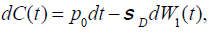(1)

and let surplus process R(t) be modeled as

(2)

Where η ≥ δ.

Note that the Brownian motion model (continuous) of the claim process is the limit of the discrete compound Poisson model [8]. Borrowing at the risk-free interest rate is not allowed, i.e., X_t is not allowed to be negative for all t≥0, the amount invested in risky assets cannot be greater than the wealth level. Let (t) be the amount invested in risky assets.

Assume that the return process of risky asset r_i(t) for i=1,2,…,n, at time follows the [23,24]. Stochastic process: π

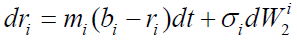(3)

Where ri the return is rate of the i-th risky asset, and wⁱ₂ (t), i=1,2,…,n, are mutually dependent standard Wiener process defined on (Ω,F,{F_t}_t≥0,P). For simplicity, it is assumed that the underlying filtration, F_t coincides with one generated by the Wiener process, that is, F_t =σ(W₂(s):0≤s≤t) and σ denotes the volatility matrix.

If m_i=m, then we have:

(4)

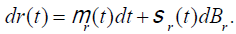
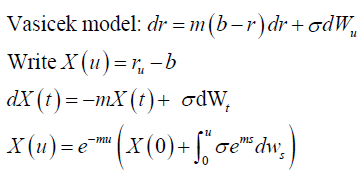
The return of investment portfolio can be described with Vasicek model as:

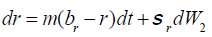(5)

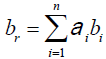
where σ_r is in instantaneous volatility of randomness measure of the return rate of investment portfolio, b_r is the long term equilibrium return rate of investment portfolio, b_r - r is the gap between its current rate of return and its long-run equilibrium level and m is a parameter measuring the speed at which the gap diminishes. The diversified portfolio consists of n types of risky investments, the fraction invested in i-th risky investment is a_i, i=1,2,…,n, or α = (α₁, α₂, ...α_n) and The return on risky asset i follows stochastic differential equation (3) and the return rate of the portfolio of risky assets is

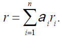(6)

The differential of the portfolio return of risky assets is

(7)

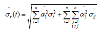
If the correlation between z_i and z_j, p_ij then the variance of the portfolio return is

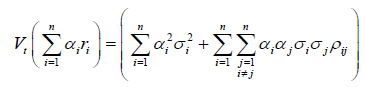(8)

And the standard deviation is

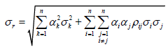(9)

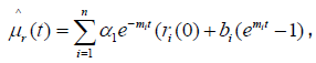
As in Momon (2004), the expected return rate of risky investment portfolio is

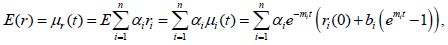(10)

Where μ_i(t) is the expected return rate of i-th risky asset at time in real world measure and r_i(0) is the return rate of i-th risky investment at t=0. Let

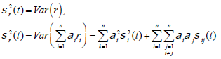(11)

where σⁱ₂(t) is the volatility of the return rate of i-th risky asset under the real world measure,

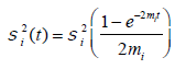(12)

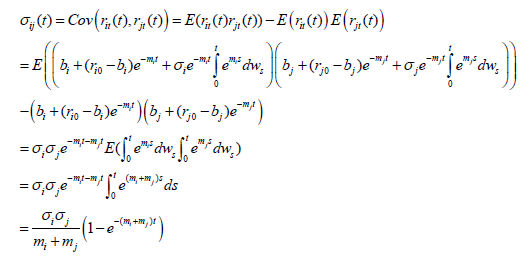
And σ_ij(t) is covariance between i-th risky asset and j-th asset under the real world measure,

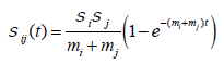(13)

For the proof of equation (13), please see Appendix A.

Based on Mamon (2004), 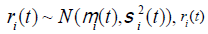also satisfies the stochastic differential equation: 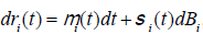, where B_i is i-dimensional standard Brownian Motion, i=1,2,…,n, and the return rate of risky investment portfolio r(t) satisfies

(14)

Let be the wealth process of the insurance company for the strategy . The insurer uses the self-financing strategy. Based on equations of (2) and (14), insurer’s wealth follows the equation below:

(15)

With a boundary condition of , and

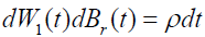(16)

where 1 {B_r(t), W₁(t) / t≥0} are standard Brownian motions on a filtered probability space (Ω,F, {F_t} t≥0, P), F_t is the P-augmentation of the natural filtration, ρ is the coefficient of correlation between B_r(t) and W₁(t) and ρ≤0; the total amount invested in risky investment, Ξ(t), is a measurable control process adapted to the filtration {F_t}_t≥0, satisfying:

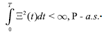(17)

Assume that α(t) is a non-negative measurable process adapted to the filtration {F_t}t≤0, satisfying equation (15), that is,

(18)

And the wealth equation (15) has unique optimal solutions of ((t),a(t),a(t))..

Extension of HJBI equation and solutions of optimal investment and retention of reinsurance

We let D_θ be the set of admissible controls by the market and let π for the set of admissible strategies ϑ=(Ξ,a,α) of the insurance company. For any T<∞, a process {θ(t) / t∈[0,T]} satisfies the condition of and (t) ≤ 1. For each θε_D, F-adapted process is a real-valued process defined on (Ω,F, {F_t}_t≥0, P) as:

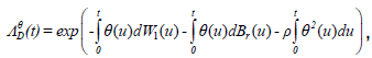(19)

By Ito’s differentiation rule, we obtain

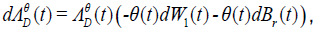(20)

Where local martingale, and satisfies For each θεΘ_D, a new (real-world) probability measure P_θ, which is absolutely continuous with respect to P, is defined on (Ω,F(T)) by

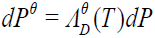(21)

The optimal problem of the insurance company can be formulated as a two-player, zero-sum, stochastic differential game as in [7]. The measure θ is the control of one player (the “market”), while the investment portfolio and retention of reinsurance (Ξa,) is the control of player two (the insurer). We define a vector process by:

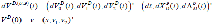(22)

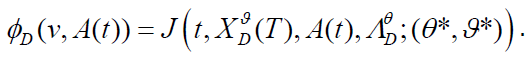
The optimization problem is formulated to Min-Max expectation for the utility of the terminal wealth. Given the initial time, t₀, the initial wealth of the insurer, X₀, the objective function over the class of admissible controls (θ,)ε(Θxπ) is given by

(23)

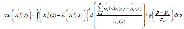
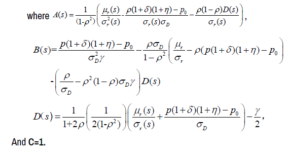
In a manner similar to the work in [25] the process A(t) is defined as

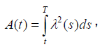
Where and μ_r(s) and σ_r(s). Satisfy equations (10) and (11), respectively. Therefore μ_r(t). in stochastic differential equation (15) can be replaced by λ(t)σ_r(t). Then performance process is defined to be dependent on A(t) and as:

Where is defined by equation (15) and is defined by equation (19).

Since 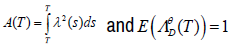, the utility does not really depend on A(T), we can transform the utility of state-dependence into the one with state-independence. Although the utility at terminal time is state-independent, it is difficult to assure that the performance process defined by equation (24) satisfies time-consistent condition at the whole state space (Θxπ).

Therefore, the defined form of 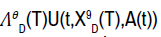may not be suitable for dynamic programming. We here assume that our performance process doesn’t satisfy time consistency and the control can be restricted only to admissible feedback control. Our objective is to min-max 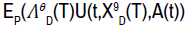for each (t, v₁, v₂), which can be proved to be the case in theorem 1. Our optimal control is not strictly optimal based on the dynamics of the process. However, for any twice continuously differential function 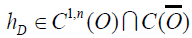, where 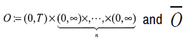denotes the closure of O, there exists a partial differential operator

According to Mataramvura and Âksendal (2008) and Bjork T, et al. [15], it is not

Difficult to get the following verification theorem

Theorem 1: Suppose that there exists a function , a function g(T,t) and an admissible feedback control such that

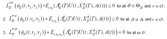
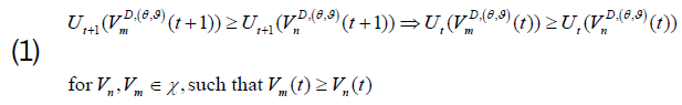
4. The value function is determined by extended HBJI defined by equation (27).

5. since , for all

6. Let K denote the set of stopping times τ ≤ T. The family is uniform integral for all

Then is an optimal control [26,27]. Proof:

First, the value function is proved to be determined by extended HBJI equation as followings. The Ito formula is applied to the performance process . Expectation of the integration yields:

Where the stochastic integral part has vanished because of the integrability Then,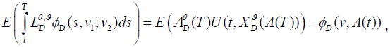

Therefore, we obtain the desired result:

Second (θ*,*) is proved to be the supremum in the value function and is proved to be an admissible feedback control as follows.

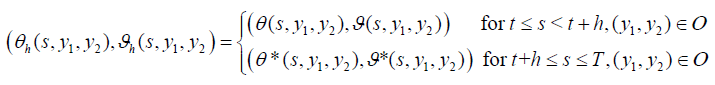
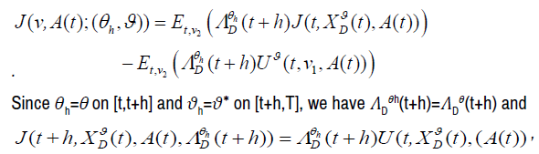
Choose (θ,)εΘ_D xπ, then, for h>0, a randomly chosen initial state (t,v₁,v₂) and define the control law (θ_h,ϑ_h) as

Furthermore, we obtain:

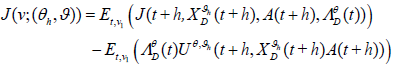
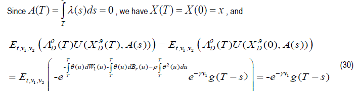
Since , we have

Then we obtain

Furthermore, from equation (23) we have .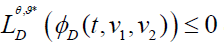

It gives us that Combining this with expression for 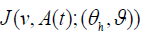above and the fact that

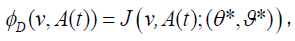
We obtain

Similarly, we obtain:

Then we have

Furthermore, from equation (23) we have . It gives us that

Combining this with expression for above and the fact that

We obtain .

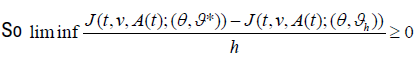
So

Then, .

This finishes the proof.

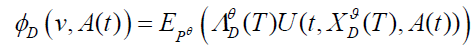
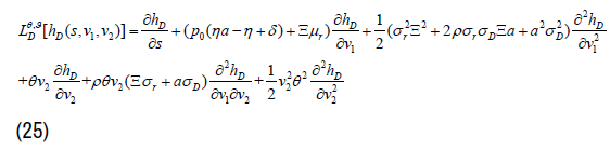
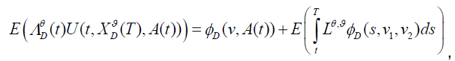
The optimal investment problem is formulated to Min-Max expectation of the exponential utility of the terminal wealth of an insurance company. Since the utility function is dependent on the present states of v=(t,v₁,v₂), the condition of HJBI equation is not satisfied. In order to obtain the optimal value function φ*(v,A(t)) and the optimal strategy (θ*,Ξ*,a*θ*), an extended HJBI equation is built as follows which is similar to Bjork T, et al. [7]

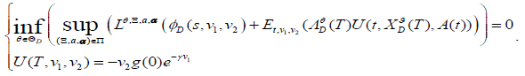(26)

A value function of exponential form as in (27) is taken to solve the equation above.

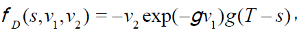(27)

Where γ is the coefficient of risk aversion, g(T-s) is an undetermined function with and the boundary condition: g(T-T)=1.

ϑ=(a,θ) and substitution of value function (27) into equation (26) result in the differential operator:

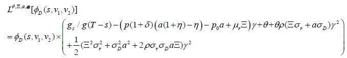(28)

We cannot show from equation (27) that

Due to the following facts: from equation (30), we will know that it is not always the case that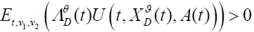

Therefore, we can only construct the extended HJBI equation because acceptable time-consistence cannot be satisfied. Combination of equation (28) and equation (26) leads to extended HJBI equation (29) as following:

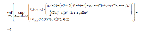(29)

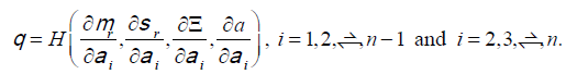
Equations (29) and (30) indicate that φD(s,v1,v2) ≠1 is the sufficient and necessary condition for the existence of optimal solutions [1]. It is necessary to make v₁ and v₂ different from zero [8]. Maximization over (Ξa,) with fixed

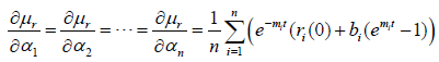
θ∈ΘD leads to the following first order conditions for the maximum point ((θ),a(θ),a(θ)) as equations of (31), (32) and (34), respectively:

(31)

(32)

(33)

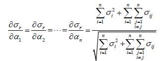
Since equation (33) can be written as following simplified form

(Please note that the following equal weights is deducted from the non-partially differential θ related term, θ and other non-partially differential θ related terms in right hand side of equation (33)) and at the same time, the constraint condition is satisfied as well.

It is implied that only when a₁=a₂=…,=a_n-1 and a₂=a₃=…,=a_n can the equation (33) hold. Therefore, we have optimal proportions of risky assets invested satisfy:

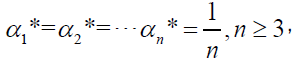(34)

That is, optimal proportion of risky assets invested is equally weighted when n≥3.

Putting equation (34) into equations of (10) and (11), respectively, we have

(35)

(36)

Although equally weighted investment strategy is usually thought of as a feasible and convenient investment strategy, it has never been demonstrated theoretically to be an optimal investment strategy under some conditions. Here our theoretical proof has demonstrated the possibility of the equal-weight investment as an optimal strategy. It is especially important to notice that equal weights can simplify greatly the optimization process.

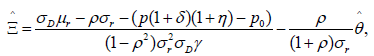
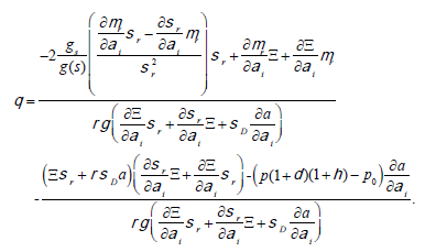
Combination of equations (31) and (32) with equations (29) and (30) and Minimization over θ result in equation (37):

(37)

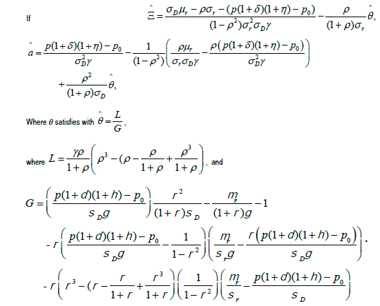
where 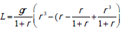, and

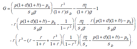
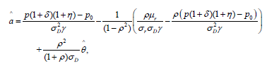
We can easily obtain the optimal solution of (t) by solving equation (37) with the equally weighted investment portfolio. Putting optimal solution of θ into equations (31) and (32), results in the optimal amount invested in risky assets and the optimal

Portion of retention of reinsurance = .

The optimal wealth process can be expressed as:

(38)

(39)

Where p is the net premium rate and p₀ is the claim loss rate.

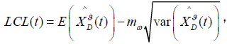
The lower control bound with (1-ϖ) confidential level is obtained by combining equations (38) and (39) as following:

(40)

Where LCL(t) is lower bound of wealth at time t(t ≤ T, and T is control period), is deviation of optimal wealth, m_ϖ is the critical value with 1(-ϖ) confidential level, while μ_r and σ_r satisfy equations (10), (11) and (34), respectively.

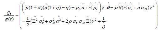
Equation (40) is obtained as following by combining equation (31), (32) and (38) with equation (28), using t instead of s and setting it equal to 0:

(41)

where

(42)

and

(43)

Integration of two sides of equation (42) and application of the boundary condition g(T,λ_T)=1 sult in the formula for g(t):

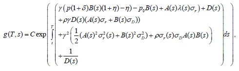(44)

We also analyze the case when â(θ,t)≤0. If â(θ,t)≤0, we should choose â(θ,t)=0 as an optimal strategy. Substitution of â=0 into equation (30) results in equation (48):

(45)

Maximization over π with fixed θ∈Θ_D leads to the following first order condition for the maximum point (θ).

(46)

With â=0 and in combination of equation (46) with equation (45), minimization over θ results in the first order condition for the minimum point, where: θ=θ.

(47)

Equation (46) and equation (47) lead to equation (48):

(48)

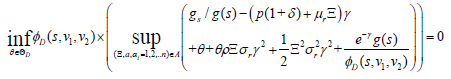
Substitution of â =0, equations (47) and (48) into equation (45) with ø(s,v₁,v₂)≠0 results in equation (49):

(49)

where

Therefore, analysis above implies the following theorem.

Theorem 2

The optimal strategy (θ*,*, θ*)=(θΞ,θ, θ) is given by equations (31), (32), (34) and (37), and the optimal value function is:

(50)

Where g(T-t) is given by equation (44).

When a(t)=0, the optimal strategy (θ*,Ξ*, θ*)=(θΞ,θ) is given by equations (47), (48) and (34). The optimal value function satisfies equation (50) where g(T-t) is given by equation (49).

Results and Discussion

Numerical analysis

The data of annual return rate of S & P 500, Treasury Bonds and Treasury Bills in U.S. from 1965 to 2014 is used in multi-variate Vasicek model. The results are displayed in Table 1. Please note that Table 1 includes the estimated values of three parameters and asymptotic errors of both Vasicek models [28].

For other data, please see Table 2. Table 3 lists optimal solutions of amount invested in risky assets, Ξ*, portion of retention, a₁* and proportions of stocks, Treasury Bonds and Treasury Bills a₁*, a₂* and a₃*. Table 3 lists the optimal solutions for different time t. Table 3 indicates that the optimal amount invested in risky assets first decreases and then increases with time, but the optimal portion of retention first increases and then decreases with time. Of course, the optimal solutions can be obtained for other terminal time T. Since insurance business is generally on-going business, which means that the life time is uncertain, it is important to obtain the optimal solutions for varying terminal time. In the following section, sensitivity analyses are carried out to the changes of the important parameters.

Varying parameters of σ_D, η and γ

Figure 1(a) displays the change pattern of time-varying correlation among risky assets invested. Figure 1(b) through (g) shows the change patterns of optimal solutions of the amount invested in risky assets and the optimal portion of the retention for different values of the volatility of claim loss, σ_D, the rate of (e) indicate that increase in the rate of reinsurance cost will greatly decrease the optimal amount invested in risky assets but greatly increase optimal portion of the retention. Figure 1(f) and Figure 1(g) show that both optimal amount of investment and optimal retention decreases with the increase of risk aversion, which is intuitive (Figures 1a-1g).

Varying parameters of σ_i and b_i,i=1,2,3.

Figures 2(a) through (d) display the change patterns of optimal solutions of the amount invested in risky assets and the optimal portion of the retention with the change of volatilities and the means of long term return of risky assets invested, σi and bi,i=1,2,3. Figures 2(a) and (b) indicate that both optimal reinsurance cost, η, and the coefficient of risk aversion, γ Figure 1(b) and (c) indicate that both the optimal amount invested in risky assets and the optimal portion of the retention decreases with the increase of the volatility of claim loss. The increase of the risk of claim loss tends to make the insurer more willing to increase reinsurance and put less funds in risky assets. Figure 1(d) and amount invested in risky assets and retention portion are greater when the volatility of the return of the stocks, Treasury Bonds and Treasury Bills decrease 10%, respectively; especially they are much more sensitive to the increase in the volatility of the return of stocks and Treasury Bonds than that of Treasury Bills, that is to say, lower volatility of the return of risky assets invested will encourage insurers to put more funds in investment, and more remains for retention of reinsurance. Figures 2(c) and (d) indicate that the optimal amount invested in risky assets increases and the optimal portion of the retention also increases when the means of long term return of the stocks, Treasury Bonds and Treasury Bills increase 10%, respectively; the optimal amount of stocks and Treasury Bonds are much more sensitive to the change of the means of long term return of stocks and Treasury Bonds than to that of Treasury Bills; and the optimal retention is also sensitive to the means of long term returns of all of three kinds of long term risky assets (Figures 2a-2d).

Figure 3(a) through Figure 3(d) display the change patterns of optimal amount investment and optimal retention portions when the correlation coefficient between investment and investment return rate of long term and volatility changes. Figure 3(a) through Figure 3(d) show that the optimal amount of risky investment decreases with the increase of correlation coefficient between investments and claim loss. However, optimal retention portion of reinsurance at first increases with the increase of correlation coefficients and then decreases with the increase of correlation coefficients (Figures 3a-3d).

Conclusion

In this paper, the optimal decision of investment and reinsurance is studied with time-inconsistence under the stochastic differential game framework. Multiple risky assets constitute investment portfolios; the returns of these risky assets follow multi-variate Vasicek model with time-varying correlation; claim losses are correlated with these risky assets. The solution to the extended HJBI equation results in dynamical optimal solutions for the amount invested in risky assets, the optimal portion of the retention and optimal proportions of all risky assets invested. A dynamical optimal bound is built for monitoring and predicting the optimal wealth level. The numerical analyses are carried out under the proposed model. The sensitivity analyses indicate that the optimal amount invested in risky assets in the proposed model are sensitive to most of the parameters except the volatility and the means of the Treasury Bills return at the long-run equilibrium; the optimal portion of the retention is sensitive to all of parameters The volatility and the means of long term returns of all three kinds of risky assets. Our sensitive analysis results are consistent to intuitions, and this demonstrates the effectiveness of our proposed model. Importantly, the investment with equally weighted risky assets can be an optimal strategy. The proposed model can be easily applied in very high dimension investment portfolio.

Appendix

We calculate the time varying covariance of σ_ij (t) of the return of stocks and bonds. In a manner similar to Korn and Koziol (2006), and Mamon (2004).

In the following, we calculate the time varying covariance, σ_ij (t), By Itô isometry, we have:

References

1. Browne, Sid. “Optimal investment policies for a firm with a random risk process: exponential utility and minimizing the probability of ruin”. Math of Oper Res 20 (1995):937-958.

Google Scholar, Crossref

2. Hipp, Christian and Michael Plum. “Optimal investment for insurers”. Insurance: J Math Econ 27 (2000):215-228.

Google Scholar, Crossref

3. Liu, Chi Sang and Hailiang Yang. “Optimal investment for an insurer to minimize its probability of ruin”. North Amer Actuarial J 8 (2004):11-31.

Google Scholar, Crossref

4. Korn, Ralf. “Worst-case scenario investment for insurers”. Insurance: J Math Econ 31 (2005):1-11.

Google Scholar, Crossref

5. Bai, Lihua and Junyi Guo. “Optimal proportional reinsurance and investment with multiple risky assets and no-shorting constraint”. Insurance: J Math Econ 42 (2008):968-975.

Google Scholar, Crossref

6. Cao, Yusong and Nianqing Wan. “Optimal proportional reinsurance and investment based on Hamilton-Jacobi-Bellman equation”. Insurance: J Math Econ 45 (2009):157-162.

Google Scholar, Crossref

7. Mataramvura, Sure and Bernt Øksendal. “Risk minimizing portfolios and HJBI equations for stochastic differential games”. Stochastics: An Inter J Prob Stochas Proc 80 (2008):317-337.

Google Scholar, Crossref

8. Zhang, Xin and Tak Kuen Siu. “Optimal investment and reinsurance of an insurer with model uncertainty”. Insurance: J Math Econ 45 (2009):81-88.

Google Scholar, Crossref

9. Mao, Hong, James M. Carson, Krzysztof M. Ostaszewski, Yan Luo and Yuling Wang. “Determining the insurer’s optimal investment and reinsurance strategy based on stochastic differential game”. J Insur Issue 39 (2016):187-202.

Google Scholar, Crossref

10. Hong, Mao, Ostaszewski Krzysztof, Yuling Wang and Zhongkai Wen. “Determination of optimal contribution rate and optimal investment portfolio of defined benefit pension plan under the expected shortfall constraint.” Pub Risk Manag: Persp Theory and Pract (2016).

Google Scholar 

11. Mamon, Rogemar S. “Three ways to solve for bond prices in the Vasicek model”. J Appl Math Deci Sci 8 (2004):1-14.

Google Scholar 

12. Korn, Olaf and Christian Koziol. “Bond portfolio optimization: A risk-return approach”. J Fixed Income 15 (2006):48-60.

Google Scholar, Crossref

13. Øksendal, Bernt, Agnes Sulem and Tusheng Zhang. “A stochastic HJBI equation for optimal control of forward-backward SDEs”.  (2016):435-446.

Google Scholar, Crossref

14. Podolskij, Mark, Robert Stelzer, Steen Thorbjørnsen and Almut ED Veraart, eds. “The Fascination of Probability, Statistics and Their Applications”. In Honour of Ole E. Barndorff-Nielsen. Springer (2015).

Google Scholar

15. Bjork, Tomas, Mariana Khapko and Agatha Murgoci. “On time inconsistent stochastic control in continuous time”. Fin and Stochastics 21 (2017):331-336.

Google Scholar

16. Yang, Hailiang and Lihong Zhang. “Optimal investment for insurer with jump-diffusion risk process”, Insurance: J Math Econ 37 (2005):613-634.

Google Scholar, Crossref

17. Mao, Hong and Zhongkai Wen. “Optimal dynamic insurance price and investment portfolio of an insurer with multi-dimensional time-varying correlation”. J Quant Eco Forthcoming (2016).

Google Scholar, Crossref

18. Browne, Sid. “Stochastic differential portfolio games”. J Applied Prob. 37 (2000):126-147.

Google Scholar, Crossref

19. Korn, Ralf and Frank Thomas Seifried. “A worst-case approach to continuous-time portfolio Optimization”. Radon Ser. Comp Appl Math 8 (2009):327-345.

Google Scholar, Crossref

20. Korn, Ralf, Olaf Menkens and Mogens Steffensen, “Worst-case-optimal dynamic reinsurance for large claim”. Eur Actuarial J 2 (2012):21-48.

Google Scholar, Crossref

21. David Promislow S., and Virginia R. Young. “Minimizing the probability of ruin when claims follow Brownian motion with drift”. N Am Actuar J 9 (2005):109-128.

Google Scholar, Crossref

22. Aase, Knut K. “The investment horizon problem: A resolution”.  NHH Depart of Fin & Manag Sci Disc Pap (2009).

Google Scholar, Crossref

23. Vasicek, Oldrich. “An equilibrium characterization of the term structure”. J Math Econ 5 (1977):177-188.

Google Scholar, Crossref

24. Lim, Byung Hwa., and Yong Hyun Shin. “Optimal investment, consumption, and retirement decision with disutility and borrowing constraints”. J Quant Fin 11 (2011):1581-1592.

Google Scholar, Crossref

25. Musiela, Marek and Thaleia Zariphopoulou. “Portfolio choice under dynamic investment performance criteria”, J Quant Fin 9 (2009):1-19.

Google Scholar, Crossref

26. Bielecki, Tomasz R., Igor Cialenco and Marcin Pitera. “On time consistency of dynamic risk and performance measures indiscrete time”. Working paper 2014.

Google Scholar

27. Fleming, Wendell H., and Raymond W Rishel. “Deterministic and Stochastic Optimal Control”. Spinger-Verlag New York, Inc. (1975).

Google Scholar

28. Gourieroux, Christian and Joann Jasiak. “Financial Econometrics”. Princeton, NJ: Princeton University Press. (2001).

Google Scholar