The Effect Of Exogenously Induced Magnetic Fields On Neurotransmitter Dynamics

Manuel Rivas^1* and Marina Martinez-Garcia^2
*Correspondence: Manuel Rivas, Department of Chemical Engineering, Polytechnic University of Catalonia, Spain, Email:

Keywords

Exogenous electromagnetic fields; Induced cell membrane magnetic field; Faraday cage; Hall effect; Electric conductivity tensor non-zero off diagonal components

Introduction

To this day the question of whether it is possible for a biological process exposed to an exogenous electric or magnetic field to generate a response signal in the organism distinguishable from background noise is still being debated [1-3].

The lack of knowledge that existed in the first electrophysiological studies on the nonlinear membrane phenomena that underlie all manifestations of electrical excitability, on the one hand, and the lack of a theory capable of quantitatively describing the flow of electrical current in tissues in vivo or in vitro beyond the limited possibilities of the one dimensional and linear cable theory, prevented the analysis, more in depth, of this type of experiments within the framework of endogenous and exogenous EM fields [4].

Later, more realistic concepts of multidimensional structure and mathematical models of three dimensional, homogeneous and isotropic cables were introduced, which served as the basis for numerous later works. In contrast to classical one dimensional cable models, in the new concept of three dimensional structures, the intracellular and interstitial spaces share the same volume on a relatively microscopic scale [5]. The high degree of interconnection that brain tissue presents suggests considering the intracellular space as a single continuum, simply connected. The same can be done with the interstitial space. The development of this idea leads to the so called bidomain theory in electroencephalography. This approach insists on the study of the potential and current fields generated in each domain by a transmembrane potential field which is often assumed to be given [6].

From the experimental results it can be deduced, not only the marked anisotropy of the brain, but also its unequal anisotropy [7]. The degree of anisotropy of the intracellular space is different from the degree of anisotropy of the interstitial space, which has important consequences on the flow of electrical current in the tissue. In addition to uneven, the anisotropy of the brain is not uniform. The non-uniformity affects both the electrotonic propagation of the polarization and the propagation of the magnetic field [8].

This uneven and non-uniform anisotropy should be taken into account in mathematical models designed to describe the flow of electromagnetic fields in the brain. But, as Sanz-Leon et al. [9] point out, a mathematical theory has not yet been formulated that can reflect at an electrophysiological level the effects of the numerous spatial scales of structural discontinuity that emerge from the histological study of the brain.

It is possible to distinguish three different, although not mutually exclusive, approaches to the problems posed by the study of the flow of electrical current in tissues [10,11]:

• As a biological tissue is not a completely ordered structure and as the variability of local morphological characteristics is generally very evident, one idea that prevails is to develop statistical models of the flow of electric current, using the methods and results of the theory of stochastic processes with parameters distributed in space.

• As a biological tissue presents a certain degree of morphometric regularity that is also very evident (in the dimensions, shape and arrangement of cells and other elements), another attractive idea is to postulate a regular geometry that is somehow related to the tissue structure, but simple enough to allow the solution of the field equations that describe the flow of electric current.

• As the results of the measurement operations can be interpreted on the basis of averages, a third way of approach that is naturally imposed is to use averaged fields and to construct averaged forms of the field equations to describe the tissue from the electrophysiological point of view.

The stochastic approach is the one that has received the least attention, until now, in electrophysiology. It has been developed for the study of heterogeneous physical systems, fundamentally for the analysis of elastic and dielectric properties, EM wave propagation and mass transport processes. Even though the media to which the stochastic approach has been applied are much simpler than biological tissues, the development of the theory presents considerable mathematical difficulties [12].

The approach based on idealizing the geometry of the tissue is the one that, until now, has been most used in electrophysiology. The different applications of the cable theory in the study of electrical current flow in the brain are included, along with other models, in this category [13].

We will use the approach based on the theory of averaged fields. The field equations obtained must be valid for any geometry, so the results obtained with regular geometry models must satisfy them. In a way, the averaging field approach is intermediate between models based on regular geometry and stochastic models. But all three methods of dealing with the question of electrical current flow in tissues lead to the introduction of unspecified parameters that must be determined experimentally.

In this paper, we present a theoretical model of the interstitial induced magnetic field determined from the effect of exogenous electric fields on cell membrane. Our model is based on electrically active interstitial and intracellular media represented by conductivity tensors with non-zero off diagonal terms. Such conductivity tensors can arise in spaces associated with a complicated geometry, like the synaptic cleft.

We propose a physic mathematical framework that maintains a well specified connection with the morphological and bioelectric properties of the brain tissue, but at the same time presents behaviour simple enough to be able to solve the field equations from the corresponding nonlinear partial differential equations. The way to contemplate these requirements (to a certain extent antagonistic) is to identify the tensor fields of conductivity of the tissues, which allow the development of an averaged field theory. We shall first review the standard calculation of the potential and magnetic field of a single cell membrane, and then show how this calculation can be generalized to describe the electric potential in the synaptic cleft. Finally, a summary of the bidomain theory is presented, considered as an extension of the three dimensional cable models.

Physical Derivation of the Model

In this section, we describe the classical view of the fields required to describe charge transport in the brain, at the microscopic scale (d). For the range of frequencies associated with the exogenous electrical activity and the applied stimulatory pulses, the electric field generated by self-induction is generally two to three times less than the order of the electric field generated by charge separation [14]. Therefore, until now when dealing with the issue of the effect of exogenous fields, the magnetic contribution to the electric field was neglected, putting (eliminating the contribution of the partial derivative of the potential vector with respect to the time). This is the reason why the effect of the magnetic field on moving charge carriers was also neglected. Next, we will explain the classical development in more detail to determine under what conditions the simplifications made are no longer valid.

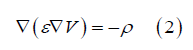
Let ε be the d-scale electrical permittivity (ε can vary from one point to another) and ρ be the charge density, the potential V satisfies Poisson's equation:

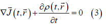
The local point current density and the local point charge density verify the continuity equation:

On the other hand, on the d scale the following generalized form of Ohm's law holds

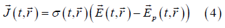
where σ (t, r) is the punctual local conductivity field (just like ε (t, r) , it could vary from one point to another and eventually, from one instant to another. The field (t ,) is the so called Planck field, associated with charge carrier concentration gradients [15]. As σ, ρ and depend on the concentrations of tissue electrolytes and, therefore, on the local geometry of the tissue at d scale, the local punctual expression Eq. (4) of Ohm's law is, in fact, much more complicated than it appears from the way it was described. Thus, the simplifications made in the classical approach to these questions could no longer be valid and we could not neglect the magnetic contribution to the electric field; and, under suitable conditions, we could not neglect the effect of the magnetic field on charge carriers [16,17].

The variation of an electric field produced by the displacement of an electric charge is always accompanied by a magnetic field [18]. While the electric charge is at rest, there is only an electrostatic field; but a magnetic field appears as soon as the charge begins to move. It can be stated even more: The magnetic field created by the movement of an electric charge will be more intense if the charge is greater and if it moves faster [19].

The working hypothesis is that whatever way the exogenous electromagnetic field acts on the cell, it does so primarily through its action on the cell membrane. The internal cavity of any conductor in equilibrium in an electric field has a constant potential and therefore a zero electric field. This is what is called a Faraday cage, which protects all the bodies enclosed in it from electrical influences. The specific electrical characteristics of the living cell (Faraday cage) and the relatively small magnitude of exogenous EM fields mean that it is not possible for this field to interact with the cell through interaction with the charged particles or the electric dipoles inside it. Thus, it is natural to consider that the EM fields could act on the cell through local changes of charge in the membrane [20,21].

The effects of EM fields on cells are attributed to a series of main mechanisms:

• Charge polarization,

• The significant orientation of permanent dipoles that cause topographical changes of molecules,

• Diffusion and movement of charges, ions that can bind or separate from proteins,

• Production of membrane receptor or ion channel clusters,

• Voltage sensitive enzymes are a special case of electroconformational coupling of protein channels [22-24]. Specifically, regarding the conformational changes in the membrane, some studies specify that the changes occur especially in the ion channels and the enzymes associated with the membrane [25,26]. These proteins, when subjected to the EM field, have a tendency to modify their orientation. But due to the very configuration of the transmembrane proteins, it is very difficult for them to rotate inside the membrane and dissipate the Debye relaxation energy [27]. The combination of conformational changes and ionic translocation creates a non-linear response to weak EM fields manifested by the generation of harmonics, creating electrical amplification phenomena [28,29].

Some specific cell membrane proteins can be arranged as a kind of electric amplifiers, such as is used in electronics [30]. These cell membrane proteins work like a Hall effect transformer [31]. A Hall effect current transformer consists of a coil of cable located next to one or more other coils, and that is used to join two or more alternating current circuits, taking advantage of the induction effect between the coils. The variation of the intensity of current in a coil (primary coil) gives rise to a variable magnetic field. This magnetic field causes a variable magnetic flux that passes through the other coil (secondary coil) and induces an electromotive force in it, in accordance with the Faraday-Henry law [32] Saleh et al. [33] have studied the conductivity tensor and Hall effect in magnetic conductors. They derived the conductivity tensor due to anisotropic scattering of electric carriers in a magnetic conductor. However, even today a quantitative theory for the spontaneous Hall effect has not been given so far [34].

The transformation ratio of an electrical transformer is defined as the ratio of the voltages at the terminals of the secondary and primary. If we consider an ideal transformer (without losses and, in particular, without resistance in the secondary or the primary), the voltages are null V₂=V₁=0 in direct current (DC), and the ratio is not defined. In fact, the primary has a resistance that intervenes when the frequency is low enough: the primary becomes above all resistive (and not inductive), the current passing through it becomes independent of the frequency; however, the secondary voltage V₂ is proportional to the frequency and tends to zero with it. Therefore, the transformer does not work in DC, nor when the frequency is too low [35].

If we consider a quasi-static regime, there would be an easily calculated potential difference between the outer and inner sides of the membrane, let's call it ΔV (volts). In this case the membrane would be driven by exactly the charge they would have accumulated if they were connected at ΔV (volts), and therefore by an identical average current [36]. If the capacitance of the membrane were C, it would have accumulated a charge Q=C·ΔV, in an average time τ=R·C (where R is the resistance). The average current would be This approximation is valid for the study of the potential difference created between the external and internal faces of the membrane; where the instantaneous currents, although tiny, comply with the above laws [37]. From the point of view of their absolute magnitude, the electrical potential differences that are generated across cell membranes are small, usually a few tens of millivolts. However, due to the small thickness of the membrane, the electrical gradient is enormous. Thus, for a cell membrane with a potential difference of 70 millivolts and a thickness of 3.5 nanometers, the resulting electrical gradient is 200,000 volts per centimeter.

At this point we will determine the effect of this induced magnetic field on the trajectory of a protein released into the extracellular space. Our particular case would be that of a magnetic field B generated by a current distribution in concentric layers perpendicular to the axial plane of the cytoplasmic membrane (let's assume for the explanation the plane of the page) [38] for this case we would have the configuration of Figure 1.

The existence of a uniform (or quasi-static) induced magnetic field in the synaptic cleft would also explain the impossibility of neurotransmitter accumulation in this region. We know that magnetic field lines cannot be open, sinceeverywhere (there are no magnetic charges), so field lines have zero ends, unlike electric field lines, which end on charges (in electrostatics) [39]. Field lines are necessarily closed (except, perhaps, for a set of null measure, such as the axis of a solenoid) [40]. The particle describes an arc of circumference in this region. Since it is a closed figure, it must intersect the border of the region at two points (or at none). Any particle that enters this region will leave after making less than one revolution. In general, it is impossible to confine a charged particle (or an electric dipole) coming from the outside (in this case the neurotransmitters stored in the vesicles of the presynaptic neuron) without losing energy in a region where there is a uniform (or quasi-static) magnetic field.

There are many previous studies that provide experimental values given in values associated with electric field magnitudes instead of magnetic field language. From now on we will try to state the above results in electric field language. A pure magnetic field in a certain reference system is transformed into an electric field in another (or a combination of magnetic and electric field). In both systems, the force is the same but not its interpretation (electric or magnetic). In our case, we have an electric dipole with linear velocity . In this reference system of point O (midpoint between the centers of the positive and negative charge of the dipole), the magnetic field is relativistically transformed into an electric field which tries to move point O in the direction of E ; causing a change of its linear velocity [41]. In the following lines we will take advantage of the Galilean transformation explained above to develop the problem in terms of electric field, more specifically in terms of electric potential.

The action of the electric field on charged particles is trivial, but not so much the action on neutral bodies, which is fundamental in our argument since most proteins are neutral. So, the first question is how can neutral bodies respond to an electric field? Because such particles are not point like, and the field acting on them is not uniform [42]. A neutral body, in an electric field, is polarized (by influence). If the field is not uniform, the positive and negative charges are subjected to forces of different intensity, which are not compensated, the bodies always move towards the region of the intense field, whatever the sign of the field (or vibrate if these bodies are part of structures that prevent their free movement) (Figure 2) [43].

For the case of the induced electric dipole, given a field tube that ends at infinity, the electric flux through this tube is the same whatever its section. Consider the cross section of the tube for a sphere of radius R; let S_R be its area. Since the total charge is zero, the mean field E_R at distance R decreases at least as a dipole field

So, we obtain:

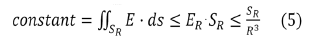
It is necessary that S_R increases at least as R³, which is obviously impossible, since S_R cannot exceed the area of the sphere (4πR²). It is thus understood why the field tubes of such charge distributions widen and then "turn around". There can therefore be no more than a numerable set of field lines that go to infinity if the total charge is zero see (Figure 3).

This means that although the transmission of the field through neutral bodies is theoretically possible, the electric field created by the neutral body is strictly local (i.e., it is approximately zero in areas far away from its localized finite sources) [44]. Under these conditions we can apply the Helmholtz theorem and the solutions to the problem will therefore have physical significance. So, if such neutral particles were contained inside compact structures where the distance between them was minimal (as in the synaptic cleft volume), an effective transmission of the field would occur [45].

Mathematical Derivation of the Model

General electrical conductivity tensor

The problem consists of calculating the resulting electric potential in the membrane when applying an external electromagnetic field. This is an electromagnetic problem with Neumann boundary conditions that can be solved from Maxwell’s equations. We represent by R the region of space occupied by the brain. The bidomain theory postulates the existence of two overlapping continuums at each point P of R and for each instant t: the intracellular continuum (subscript i) and the interstitial continuum (subscript e). Likewise, it postulates that these continuums are electrically connected to each other through a system of excitable membranes, a system that is also supposed to occupy the entire R region. Two scalar fields ϕ_i and ϕe are introduced to represent the electrical potential in the intracellular continuums and interstitial, respectively. The membrane system is assigned, at each point of R for each instant, the field V_m=ϕ_i-ϕ_e which is interpreted as a transmembrane potential field [46].

Two electric current density vector fields and (intracellular and interstitial, respectively) and a scalar electric current density J_m that is assigned to the membranes are then introduced. The first problem that arises is that of justifying in an operational way (that is, in principle accessible through electrophysiological measurements), the introduction of the superimposed continuums together with the corresponding fields.

In the bidomain theory, the continuity equations of the electric current are postulated in each continuum or domain:

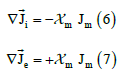
where is the fraction of membranes at the point considered in the bidomain (that is, the area of membranes connecting the intracellular and interstitial spaces per unit volume of tissue).

The second problem, then, is to adequately justify these two equations. To connect the electric current density with the potential gradient, the constitutive equations, characteristic of the intracellular and interstitial continuums, are postulated, under the form of Ohm's law for an anisotropic volume conductor [47].

These equations have been formulated by taking the vectors , and according to the main directions of the conductivity tensors of one and the other continuum (assuming that the main directions are the same for both media, the interstitial and the intracellular).

The third problem is to justify Eqs. (8) and (9) from the equations of electromagnetic theory, taking into account the irregularity of the distribution of the fields and the complexity of the originating boundary conditions, on the scale d because of the tissue structure. In the bidomain theory, the main conductivity coefficients 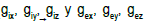are introduced, as well as the current densities and , referred to the total tissue space. Subsequently, the volume fractions f_i and f_e are made to appear (the membranes are assumed to have zero volume) to connect the coefficients g with the coefficients σ:

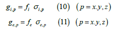
In turn, the conductivity coefficients σi and σe refer each one of them, to the corresponding continuum. They express the intrinsic conductivity properties, regardless of the volume fraction that this continuum occupies.

But, as by definition, the current densities are referred to areas, in the conductivities the area fractions should appear instead of the volume fractions f:

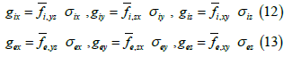
Here, represents the fraction of area occupied by phase u on a flat surface (at scale f) parallel to the coordinate axes x and y, centered at point P of the bidomain to which said fraction of area is assigned area. An analogous interpretation has the other two area fractions at that same point of the bidomain: and .

In the bidomain theory it is postulated, for each point of the bidomain:

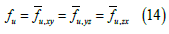
where u represents either i or e (it is enough to postulate Eq. (14) for one of the two continuums, in that case it is also verified for the other, since the sum of the volume and area fractions are always equal to 1) So, both the intracellular (i) and interstitial (e) conductivities have been represented as diagonal tensors

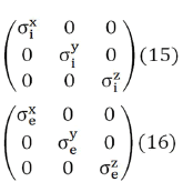
The conductivity tensors in Eqs. (15) and (16) expressed in cylindrical coordinates takes the following form,

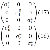
The ionic mobility both inside the cell and in the extracellular space is quite reduced, compared to an aqueous solution. Ion pathways within the cell are blocked by contractile proteins, the sarcoplasmic reticulum, mitochondria, and other structures, as well as by electrical interactions with the relatively immobile constituents of the cytoplasm (cytoskeleton and microtrabecular meshwork) [48].

Ion pathways in the extracellular space are blocked by the many fibers in the connective tissue and various macromolecular forms, as well as by the membranes of cells (other than neurons) found in that space (capillaryassociated, immune system…). The passage of ions through biological membranes generally occurs through localized structures, especially ion channels. On average, a width of 4 Å (0.4 nm) can be assigned to a channel and a distance of 150 Å (15 nm) between two channels. Taking into account the selectivity of the channels, for the same ionic type, the distance between two channels of the same type will generally be considerably gr eater [49].

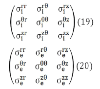
As a consequence of this structural complexity in brain tissue, the conductivity tensors of the intracellular and extracellular domains would require a more complete formulation, containing non-zero off diagonal terms like Eqs. (19) and (20).

The induced magnetic field

The Biot-Savart law allows calculating the magnetic field produced by an electric current,

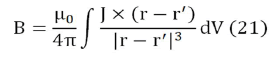
which can be rewritten as

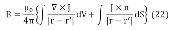
The most general possible form for B is B=B (r,θ,z), that is, in cylindrical coordinates. The considered system is invariant with respect to rotations and displacements around z axis, so the source terms in the integrands in Eq. (22) can be written as.

If either σ^θr or σ^zθ is not zero, then J^θ does not vanish and there exists components of the magnetic field in the r and z directions.

In our case, the induced magnetic field exhibits cylindrical symmetry, regardless of the existence of off diagonal terms in the conductivity tensor [50,51]. Tang et al. [52] studied sub-synaptic molecular architecture in cultured rat hippocampal neurons during synaptic transmission. They observed that the gradients of protein density are aligned to the densest receptor areas, suggesting a nanocolumn model, optimizing the potency of neurotransmission. This experimental data contributes to guarantee the electromagnetic cylindrical symmetry in the synaptic cleft [53].

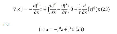
We will now derive analytic expressions for the magnetic field based on Eq. (22) through Eq. (24). Applying the divergence to the current density and taking into account that within the volume Ω it is zero (there are no current sources), and that, on the contrary, on the surface δΩ the current source and sink are oriented in the direction normal to the surface, the problem is defined by:

Where = (x, y, z) represents a generic point in space. In a spherical model, this problem can be solved analytically using Legendre polynomials and spherical coordinates [54]. To solve the problem using a realistic cell shape (and a general tissue fiber) the finite element method is used.

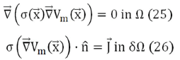
As it is sought to fulfill the first condition Eq. (25), a weight function ω is proposed that satisfies:

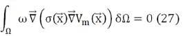
What is known as the heavy residue method, where V_m is the potential to be calculated. Applying gradient and divergence properties, expression Eq. (27) can be written as:

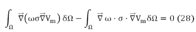
known as the weak formulation of the problem. Then, applying Green's Theorem to the first term, we get

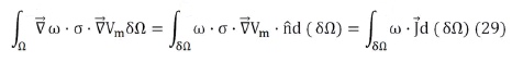
To solve these integrals, the volume is discretized into tetrahedra and a linear interpolation is applied within them (first order finite element method). The volume integral of Eq. (29) is solved for each element of the discretization, obtaining a K_e matrix (called the elemental matrix) for each tetrahedron and the assembled set of all the K_e forms the stiffness matrix K of the problem. This matrix is n×n, where n is the number of points (vertex of the tetrahedra) of the discretization. In this way, the problem is linearized, remaining in the form KU=F, where U is the unknown vector formed by the electric potential at the vertices (of n×1) and F is the independent vector. It is possible to show that F is made up of all zeros except +I and I in the elements located at the current injection points [55]. Where I is the charge per unit time and per unit area that crosses the face of the tetrahedron.

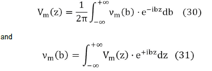
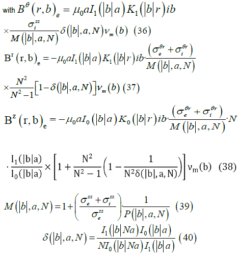
From this approach, Roth et al [56] expressed the transmembrane electric potential (V_m) in terms of its Fourier transform using cylindrical coordinates which does not depend on r , z , r and z (Eqs. (30-35)). Then they derived analytic expression for the induced magnetic field in the interstitial media () where depend on and (Eqs. (36-40)) [57,58].

Starting from the transmembrane potential V_m (z) using its Fourier transform ν_m (b),

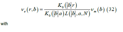
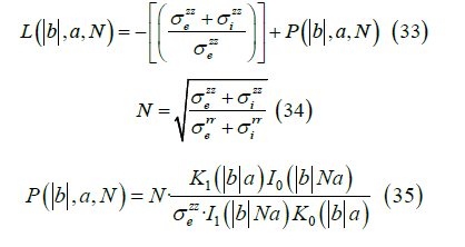
We obtain the Fourier transform of the external potential ν_e ( r,b ) where a is the width of the cell membrane,

The Fourier transform of the magnetic field (r > a) , is given by

An electric dipole can be assumed to be formed by two-point charges (±q) located at the ends of a short rod of length , where p is the electric dipole moment. An electric dipole, whether it is a localized current or possesses an intrinsic moment, experiences the action of an external magnetic field, which tends to move and orient it. The dipole experiences a force and a moment of a force and has a certain potential energy.

It is possible to derive the expressions for the force and torque on the dipole from the Lorentz force. For the case of a constant momentum dipole, it can be transformed into a more manageable expression. If, in addition, the dipole is not submerged in a current distribution, as is the case of a neurotransmitter released in the synaptic cleft, the force can be expressed as

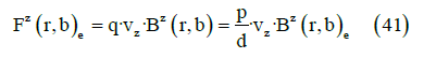
where v_z is the speed in the z axis.

Let us suppose an electric dipole initially at rest in a vertical, uniform and variable (for example, linearly increasing in time) magnetic field. The movement of the dipole depends on the configuration of the field, not the magnetic one, since it remains constant, but the induced electric one, and, consequently, the electric potential (V_e ) that generates the field.

Although the magnetic field is not conservative, the electromagnetic field as a whole is conservative. Thus, if we apply the principle of conservation of energy for a dipole in a region of potential V_e, the potential energy is transformed into kinetic energy

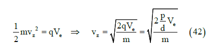
where m is the dipole mass. From Equations (41) and (42) we obtain

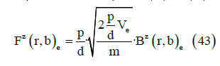
This is the key point of this paper. Our analysis provides a local mechanism for generating local magnetic field lines patterns described by a generalized conductivity tensor with off diagonal components that were previously thought to exist on only a much large scale. It is the reason we claim that an exogenous electromagnetic field can produce a biological effect in living tissues.

Time varying electric fields are not associated with charges, but with temporary variations in the flux of the magnetic field. For induced electric fields, due to the variation of the magnetic flux, the induced electromotive force (emf) is non-zero. Therefore, one can speak of induced emf for a given path without the need for it to coincide with a physical circuit.

The magnetic field is applied in such a way that magnetic field acts along the positive direction of z-axis. According to coordinate geometry, x-axis, y-axis and z-axis are perpendicular to each other. Thus, the current carrying path is perpendicular to the path along which the magnetic field is acting. Analytic expressions for the induced magnetic flux are described in the Appendix.

Appendix

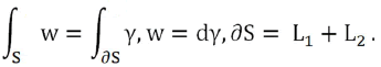
We can assume the extracellular domain of the transmembrane protein as a hemisphere. In this way we can calculate the flux of a unitary magnetic field whose direction in Cartesian components is (z,x,0) towards the outside of the quadrant of the sphere x²+y²+z²=r², x≥0, z≥0 see (Figure 4).

L₁ and L₂ semicircumferences

S₁ and S₂ semicircles

S dial quadrant

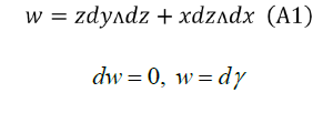
Let's find γ as simple as possible, for example,

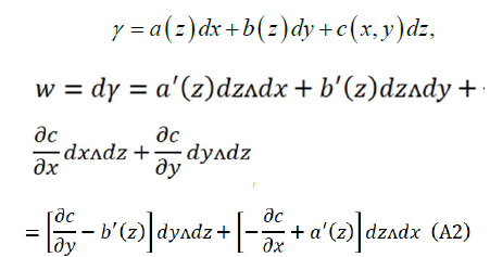
Comparing (A1) and (A2):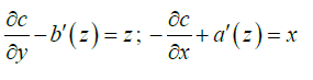

We can do a=0,c=c (x)

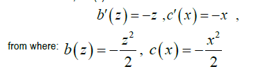
That is to say: 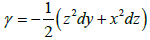is a primitive of w the most general will be of the form γ+δ, with dδ=0.

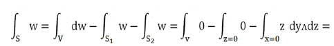
Applying Gauss's theorem: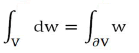

With V quadrant of ball of radius r and ∂V=S+S₁+S₂. Result

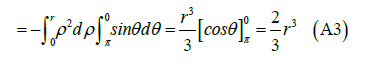
Variable change: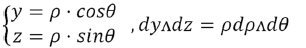

We could also calculate the magnetic flux by applying the Stokes Theorem (classical)

It has

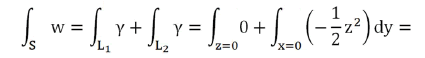
Variable change: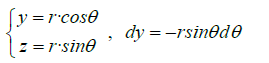

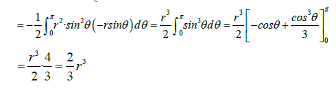
Thus, the flux of a non-unitary magnetic field of magnitude B created by a cell membrane protein (acting as a transformer-amplifier), will be

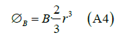
Where r is the radius of the sphere that approximates the shape of the transmembrane protein.

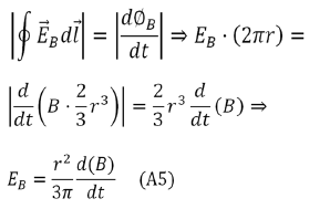
The induced electric field is tangent to this path, and because of the cylindrical symmetry of the system, its magnitude is constant on the path. Hence, we have

Discussion and Conclusion

Given the existence of off diagonal terms in the synaptic cleft conductivity tensor, then this paper proves that an exogenous electromagnetic field can induce a magnetic field in the synaptic cleft, and so the possibility to modify the neurotransmitter dynamics. The obvious question is whether such conductivity tensor occur in nature? Whether this possibility can be exploited experimentally remains to be seen.

The averaged field theory makes it possible to specify the relationship between the state variables used in the model and the peculiarities of structure and function of brain tissue. Expressing the fields and parameters at the microscopic scale as a function of the morphological properties and the tissue bioelectric and physicochemical parameters.

In our model, the anisotropy of the tissues and their non-uniformity make the use of concepts and methods of tensor analysis essential. Riemann's geometries allow translating certain electrophysiological problems into a convenient geometric language, introducing metrics defined from the emerging microscopic scale tensor conductivity fields already associated with intracellular, interstitial, active bioelectric, and passive bioelectric continuums. As a consequence, these types of models play an important role in electrophysiology, especially in relation to quantifying the effect of exogenous electromagnetic fields on specific parts of brain tissue, in particular in its effect on synaptic transmission.

Ethical Approval

Not applicable.

Authors Contribution

M.R. and M.M, wrote the main manuscript text and prepared all the figures. All listed authors have contributed significantly to the manuscript and consent to their names and order of authorship on the manuscript. Coauthors will be kept informed of editorial decisions and changes made. There is no conflict of interests involving the conduction or the report of this research.

Availability of Data and Materials

Hereby, we Manuel Rivas and Marina Martinez consciously assure that for this manuscript the following is fulfilled:

• This material is the authors' own original work, which has not been previously published elsewhere;

• The paper is not currently being considered for publication elsewhere;

• The paper reflects the authors' own research and analysis in a truthful and complete manner;

• The paper properly credits the meaningful contributions of co-authors and co-researchers;

• The results are appropriately placed in the context of prior and existing research;

• All sources used are properly disclosed (correct citation). Literally copying of text must be indicated as such by using quotation marks and giving proper reference;

• All authors have been personally and actively involved in substantial work leading to the paper and will take public responsibility for its content.

Conflict of Interest

The authors certify that they have NO affiliations with or involvement in any organization or entity with any financial interest (such as honoraria; educational grants; participation in speakers’ bureaus; membership, employment, consultancies, stock ownership, or other equity interest; and expert testimony or patent licensing arrangements), or non-financial interest (such as personal or professional relationships, affiliations, knowledge or beliefs) in the subject matter or materials discussed in this m anuscript.

References

1. Brooks, C, Hoffman B, Suckling E and Orias O. “Excitability of the Heart. Grune and Stratton. New York." (1955).
2. Cohen, D. “Magnetic Fields of the Human Body.” Physics Today 28(1975):34-43.

   [Crossref] [Google Scholar]

3. Plonsey, R. “The Nature of Sources of Bioelectric and Biomagnetic Fields.” Biophys J 39(1982):309-312.

   [Crossref] [Google Scholar]

4. Ammari, M, Jeljeli M, Maaroufi K and Roy V, et al. “Static Magnetic Field Exposure Affects Behaviour and Learning in Rats.” Electromag Biol Med 27(2008):185-196.

   [Crossref] [Google Scholar]

5. Echahgadda, I. “Changes in the Excitability of Primary Hippocampal Neurons Following Exposure to 30 GHz Radiofrequency Electromagnetic Fields.” Sci Rep 12(2022):3506-3518.

   [Crossref] [Google Scholar]

6. Feng, Y, Okamoto RJ, Namani R and Genin GM, et al. “Measurements of Mechanical Anisotropy in Brain Tissue and Implication for Transversely Isotropic Material Models of White Matter.” J Mech Behav Biomed Mater 23(2014):117-132.

   [Crossref] [Google Scholar]

7. Kenner, J. “Causes of Propagation Failure in Excitable Media. In Rensing L, Heiden U. and Mackey M. (Eds.). Temporal disorder in human oscillatory systems. Springer. Berlin.” (1986).
8. Chatelin, S, Deck C and Willinger P. “An Anisotropic Viscous Hyperelastic Constitutive Law for Brain Material Finite-Element Modelling.” Biorheology 47(2010):255-276.

   [Crossref] [Google Scholar]

9. Sanz, LP, Knock SA, Spiegler A and Jirsa VK. “Mathematical Framework for Large-Scale Brain Network Modelling in the Virtual Brain.” NeuroImage 111(2015):385-430.

   [Crossref] [Google Scholar]

10. Zykov, V and Morozowa O. “Speed of Spread of Excitation in a Two-Dimensional Excitable Medium.” Biophysics 24(1980):739-744.

    [Crossref] [Google Scholar]

11. Field, R and Burger M. “Oscillations and travelling waves in chemical systems. Wiley, New York.” (1985).
12. Zykov, V. “Simulation of a Wave Processes in Excitable Media. Manchester Univ Press Manchester.” (1987).
13. Pressler, M. “Passive Electrical Properties of Cardiac Tissues. In Zipes D and Jalife J (Eds) Cardiac Electrofisiology Saunders Philadelphia.” Clin Cardiol 14(1990):108-122.

    [Crossref] [Google Scholar]

14. Plonsey, R. “Laws Governing Current Flow in the Volume Conductor. In Nelson C and Geselowitz D. (Eds.) the Theoretical Basis of Electrocardiology.” Clarendon Press Oxford (1976).
15. Ortoleva, P and Schimdt S. “The Structure and Variety of Chemical Waves. In Field R and Burger M. (Eds.) Oscillations and Travelling Waves in Chemical Systems. Wiley New York.” (1985).
16. Zimmermann, U. “Biochim Electric Field-Mediated Fusion and Related Electrical Phenomena.” Biophys Acta 694(1982):227-277.

    [Crossref] [Google Scholar]

17. Sinha, N, Heckman CJ and Yang Y. “Slowly Activating Outward Membrane Currents Generate Input-Output Sub-Harmonics Cross Frequency Coupling Neurons.” J Theor Biol 509(2021):6535-6549.

    [Crossref] [Google Scholar]

18. Purcell, E. “Electricity and Magnetism. 3^rd edition, Cambridge University press.” (2013).
19. Jackson, JD. “Classical Electrodynamics. 3^rd edition Wiley, New York.” (1998).
20. Adey, WR. “Tissue Interactions with Non-Ionizing Electromagnetic Fields.” Physiol Rev 61(1981):435-514.

    [Crossref] [Google Scholar]

21. Aaron, RK, Boyan BD, Ciomba DH and Schwartz Z, et al. “Stimulation of Growth Factor Synthesis by Electric and Electromagnetic Fields.” Clin Orthop Relat Res 419(2004):30-37.

    [Crossref] [Google Scholar]

22. Sepersu, EH. “Stimulation of an Ouabain-Sensitive Rb+ Uptake in Human Erthrocytes with an External Electric Field.” J Membr Biol 74(1983):191-201.

    [Crossref] [Google Scholar]

23. Kell, DB. “Biosensors; Fundamentals and applications Oxford University Press, Oxford.” (1987).
24. Davey, CL. “Emerging Electromagnetic Medicine. Springer Berlin.” (1990).
25. Westerhoff, HV, Astumian RD and Kell DB. “Mechanism for the Interaction between Nonstationary Electric-Fields and Biologica-Systems. Nonlinear Dielectric Theory and Free-Energy Transduction.” Ferroelectrics 86(1988):79-101.

    [Crossref] [Google Scholar]

26. Harris, A, Spray DC and Bennet MVL. “Control of Intercellular Communication by Voltage Dependence of Gap Functional Conductance.” J Neurosci 3(1983):79-100.

    [Crossref] [Google Scholar]

27. Pethig, R and Kell D. “The Passive Electrical Properties of Biological Systems: Their Significance in Physiology, Biophysiology and Biotechnology.” Phys Med Biol 32(1987):933-970.

    [Crossref] [Google Scholar]

28. Lauger, P and Jauch P. “Microscopic Description of Voltage Effects on Ion Driven Cotransport Systems.” J Membr Biol 91(1986):275-284.

    [Crossref] [Google Scholar]

29. Robertson, B, Astumian RD and Tsong YY. “Nonlinear Effects of Periodic Electric Fields on Membrane Proteins.” Biosyst 2(1989):191-209.

    [Crossref] [Google Scholar]

30. Escobar, JF, Vaca Gonzalez JJ, Guevara JM and Garzon ADA. “Effect of Magnetic and Electric Fields on Plasma Membrane of Single Cells: A Computational Approach.” Eng Rep 2(2020):12115-12124.

    [Crossref] [Google Scholar]

31. Turlier, H and Betz T. “Unveiling the Active Nature of Living-Membrane Fluctuations and Mechanics.” Annu Rev Condens Matter Phys 10(2019):213-232.

    [Crossref] [Google Scholar]

32. Woo, BY and Wei LY. “Semiconductor Theory of Ion Transport in Thon Lipid Membranes: II Surface recombination.” Bull Math Biol 36(1974):247-256.

    [Crossref] [Google Scholar]

33. Saleh, N and Qureshi AH. “Conductivity Tensor and Hall Effect in Magnetic Semiconductors.” J Appl Phys 42(1971):4313-4315.

    [Crossref] [Google Scholar]

34. Du, ZZ, Wang CM, Sung HP and Xie XC. “Quantum Theory of the Nonlinear Hall Effect.” Nat Commun 12(2021):1-7.

    [Crossref] [Google Scholar]

35. Creff, M, Faisant F, Rubi JM and Wegrowe JE. “Surface Currents in Hall Devices.” J Appl Phys 128(2020):054501-054517.

    [Crossref] [Google Scholar]

36. Mani, RG and Von Klitzing K. “Hall Effect under Null Current Conditions.” Appl Phys Lett 64(1994):1262-1264.

    [Crossref] [Google Scholar]

37. Kobe, DH. “Helmholtz Theorem for Antisymmentric Second Rank Tensor Fields and Electromagnetism with Magnetic Monopoles.” Am J Phys 52(1984):354-358.

    [Crossref] [Google Scholar]

38. Rohrlich, F. “The Validity of the Helmholtz Theorem.” Am J Phys 72(2004):412-413.

    [Crossref] [Google Scholar]

39. Bayford, RH. “Bioimpedance Tomography (Electrical Impedance Tomography).” Annu Rev Biomed Eng 8(2006):63-91.

    [Crossref] [Google Scholar]

40. Hu, XF, Wu J and Van der Laan G. “Discontinuous Properties of Current-Induced Magnetic Domain will Depinning.” Sci Rep 3(2013):2274-2289.

    [Crossref] [Google Scholar]

41. Le, Bellac M and Levi Leblond JM. “Galilean Electromagnetism. Il Nuovo Cimento B.” 14(1973):217-233.

    [Crossref] [Google Scholar]

42. Panofsky, WKH and Phillips M. “Classical Electricity and Magnetism. 2nd edition. Dover Publications, Mineola, New York.” (1962).
43. Khokmetskii, A, Missevitch O and Yarman T. “Electric/Magnetic Dipole in an Electromagnetic Field: Force, Torque and Energy.” Eur Phys J Plus 129(2014):215-222.

    [Crossref] [Google Scholar]

44. Owen, GE. “Introduction to electromagnetic theory. Courier Dover Publications.” (2003).
45. Tsang, T. “Classical electrodynamics. World Scientific.” (1997).
46. Woosley, JK, Roth BJ and Wikswo Jr JP. “The Magnetic Field of a Single Axon: A Volume Conductor Model.” Math Bioci 76(1985):1-36.

    [Crossref] [Google Scholar]

47. Clark, JW and Plonsey R. “The Extracellular Potential Field of the Single Nerve Axon in a Volume Conductor.” Biophys J 8(1968):842-864.

    [Crossref] [Google Scholar]

48. Ganapathy, NJ, Clark JW, Wilson OB and Giles W. “Forward and Inverse Potential (Field Solutions for Cardiac Strands of Cylindrical Geometry. IEEE (Inst Electr Electron Eng).” Trans Biomed Eng 32(1985):566-577.

    [Crossref] [Google Scholar]

49. Rush, S. “On the Independence of Magnetic and Electric Body Surface Recording. IEEE (Inst Electr Electron Eng).” Trans Biomed Eng 19(1972):239-244.

    [Crossref] [Google Scholar]

50. Zuo, F. “A Geometric Method to Determine the Electric Field due to a Uniformly Charged Line Segment.” Am J Phys 83(2015):567-576.

    [Crossref] [Google Scholar]

51. Axner, Y. “Calculation of some Magnetic and Electric Fields with Cylindrical Symmetry.” Appl Sci Res 4(1995):124-136.

    [Crossref] [Google Scholar]

52. Tang, AH. “A Trans-Synaptic Nanocolumn Aligns Neurotransmitter Release to Receptors.” Nature 536(2016):210-214.

    [Crossref] [Google Scholar]

53. Hu, ZN and Lu VC. “Chiral Lipid Bilayers with Cylindrical Symmetry.” Int J Mod Phys B 19(2005):2999-3011.

    [Crossref] [Google Scholar]

54. Frank, E. “Electric Potential Produced by Two-Point Current Sources in a Homogeneous Conducting Sphere.” J Appl Phys 23(1951):1225-1228.

    [Crossref] [Google Scholar]

55. Van, der Vorst. “A Fast and Smoothly Converging Variant of BI-CG for the Solution of Nonsymmetric Linear Systems.” J Sci Stat Comput 13(1992):631-644.

    [Crossref] [Google Scholar]

56. Roth, BJ and Wikswo Jr P. “Electrically Silent Magnetic Fields.” Biophys J 50(1986):739-745.

    [Crossref] [Google Scholar]

57. Lightill, MJ. “Introduction to Fourier Analysis and Generalized Functions. London, England: Cambridge University Press.” (1990).
58. Titchmarsch, EC. “Introduction to the Theory of Fourier Integrals. London: Oxford University Press.” Chap 7 (1939).