Review Article - (2023) Volume 13, Issue 9
Received: 22-Sep-2022, Manuscript No. JPM-22-75669;
Editor assigned: 26-Sep-2022, Pre QC No. JPM-22-75669(PQ);
Reviewed: 11-Oct-2022, QC No. JPM-22-75669;
Revised: 20-Dec-2022, Manuscript No. JPM-22-75669(R);
Published:
03-Jan-2023
, DOI: 10.37421/2090-0902.2023.14.407
Citation: Kiprotich, Sheila. "Mathematical Modelling to
Determine the Velocity of the Contaminant in a Flow through a Porous
Medium." J Phys Math 14 (2023): 407
Copyright: © 2023 Kiprotich S. This is an open-access article distributed under the terms of the creative commons attribution license which permits unrestricted use,
distribution and reproduction in any medium, provided the original author and source are credited.
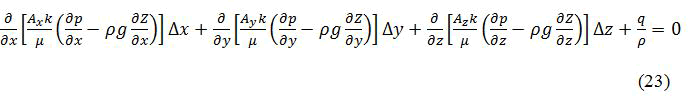
The transport of contaminants emanating from localized sources such as factories and agricultural farms in porous media, is of hydro dispersion phenomena, and has been the major subject for more than four decades. Because of industrial and agricultural activities, inorganic wastes mainly non-biodegradable substances from oil spills, human wastes, fertilizers among others, percolates through porous media and eventually find their way to water bodies and food crops in the farms. Some of these substances are harmful to human health and gets to our bodies through the water we drink or the food we eat. This research study aims to formulate a particle tracking mathematical model of contaminant flow through a porous media. The governing equation of three-dimensional concentration distribution in fluid flow through porous media has been formulated using advection-dispersion equation. This equation has been solved analytically and numerically using three-dimensional finite difference algorithm. Simulation to validate solutions is done using data from agricultural chemicals as the source point. Results confirm that the concentration of one time source of contaminant decreases as it diffuses away from the source point with respect to distance and time. The plume evolved horizontally and vertically, with peak concentration at the source, and decays further and downwards due to degradation, reaction and sorption. Particle concentration tracking shows that concentration of 100 mg/l at a point source decreases to 0 mg/l, after a distance of 300 m. For a toxic chemical like sulphur dioxide, glyphosate, and trinidol, if released from a point near borehole or food crops less than 300 m, the contaminant can be traced to the drinking water and edible parts of the crop and accumulation in the body may be carcinogenic or cause kidney and liver infections. We recommend that for water pollution minimization, and safe food crops, the source of contaminant should be more than 300 m. Additional reaction methods can be used to decompose the contaminant before reaching unwanted places.
Representative elementary volume • Accumulation • Contaminant • Mod flow• Support vector machine
FDM: Finite Difference Method; REV: Representative Elementary Volume; MF: Mod Flow; GPST: Generalized Pulse Spectrum Technique; ADI: Alternative Direction Implicit; HCU: Hydraulic Conductivities Up-scaling; SVM: Support Vector Machine; ADRE: Advection Dispersion Reaction Equation; CTRW: Continuous Time Random Walk; PT: Particle Tracking; PDF: Probability Density Function; IFD: Integrated Finite Difference; BOD: Biochemical Oxygen Demand; COD: Chemical Oxygen Demand; TDS: Total Dissolved Solid; TSS: Total Suspended solids
The transport of pollutants in the porous media, is of hydrodynamic dispersion phenomena, has been research subject for more than four decades. The agricultural activities and uncontrolled use of pesticide in agriculture cause serious damages on the environment in the area and affected groundwater [1].
Particle tracking model have become an essential tool for assessing environmental risks to groundwater resources, remediation of sulphur dioxide and agricultural inputs, engineering or the design of underground repositories of nuclear wastes, potential threat of contaminant source of drinking water well and complexity of solutes transport in subsurface systems with the occurrence of variety of chemical, physiochemical, biochemical mechanisms together with otherspatially and temporal variability and heterogeneity of hydraulic with other related dynamics such as porosity, viscosity, temperature, gradient, permeability among others within a given time (walk) frameworks [2].
Solute particles from human activities on earth, is the source of such pollutants. These contaminants reach water body with waste water drainage and reach an aquifer due to infiltration from wastes disposal sites, underground septic tanks, mine and polluted water bodies that recharge the aquifer. Solutes are transported down the stream along the flow and disperse due to combined effects of diffusion and advection with respect to time and position [3].
Most of the chemicals which are used in the refining process of the cane sugar eventually find their way into the waste residue which is the molasses. Such toxic chemicals include sulphur dioxide, hydrochloric acid, lead and other inorganic substances. These effluents are released from the industries and find their way to the water bodies downstream.
In this study, we therefore consider solute or tracer particles of sulphur dioxide and other agricultural chemicals. Such pollutants are major cause of degradation of the hydro-environment in the surface water bodies and aquifers. Solute particles of sulphur and agricultural input like fertilizer, fungicide, herbicide etc. from the source point (agricultural farms) reach the down ward region (stream) along the porous media through diffusion (dispersion) because of high concentration (diffusion) gradient within an infinite territory, contour velocity and decay sorption of the effluents in three dimensions was considered [4].
If the quantity is a mass, then the flux q is a rate of mass per area per time, and its dimensions are ML−2T−1; the metric units are kg/m2s.
Obviously, the amount of substance traversing the cross-section over which the count is performed depends on the nature of the transporting process. If this process is the passive entrainment of the substance by the carrying fluid, then the flux can be easily related to the substance concentration and the fluid velocity, as follows:
q=quantity/volume of fluid × volume of fluid/cross section area × time duration
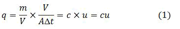
Where u is the entraining fluid velocity. This process is called advection, a term that simply means passive transport by the containing fluid. In fluid mechanics, this process used to be called convection, but the latter designation is now reserved to describe the vertical motions induced by gravity in a fluid heated from below or cooled from above. Advection is but one process by which a substance can be carried from place to place [5].
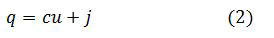
Another, important process is diffusion, whereby molecular agitation and/or small-scale turbulent motions act to move the substance randomly with respect to the mean motion of fluid. Denoting this flux by j we then write:
q=advective flux+diffusive flux
Diffusion: Diffusion is the process, or combination of processes, by which a substance is moved from one place to another under the action of random fluctuations. At the molecular level, the cause is the perpetual agitation of molecules, whereas at the turbulence level, it is advection by the turbulent eddies of the carrying fluid. Although, we can separate molecular diffusion from turbulent diffusion, it remains that in either case the impossibility of describing the details of the motions begs for a modeling assumption, called parametrization (Figure 1).

Figure 1. Diffusion
Objective of the study’s
General objective: The general objective of this study was to use contaminant transport mathematical model to track the diffusion and concentration of glyphosate in agricultural inputs and industrial wastes.
Specific objectives: The specific objectives of this study were too basically to track glyphosate contaminant transport, through porous media to water bodies and farms and use the transport model to determine concentration, distance of spread and velocity of the contaminant.
Describe the transduction dynamics of contaminant particle in its disintegration and change in concentration in plants traced to the edible parts [6].
Describe concentration of a particle with respect to decay and sorption in three dimensions.
Significance of the study
This study of a particle tracking of chemical solute of underground water through a porous medium is of every important consideration as far as the environment around us is concerned. It is mainly imperative for scientists and engineers to be aware of the possible environmental effects, in order to mitigate those effects, for examples lower the sulphur emission responsible for acid rain.
It also assists in minimizing water pollution through proper deposition of industrial wastes, sewers among others, thus reduces the hazardous effects of the contaminants causing waterborne disease, skin diseases, and other diseases like asthma, eye infection, etc.
It will also assist to formulate policies and new regulation like oxidants to control sources in order to obtain certain level of amelioration at specified receptors example proper management of dumpsites and sewage disposal of molasses residues especially in major sugar processing industries.
This also leads to greater knowledge in chemical use in agricultural produce that is proper use of herbicides and pesticides. Such knowledge helps to minimize erosion of sludge deposits in water body that can cause a blanket of material that can destroy fish, fauna and flora [7].
In this chapter, we explore contributors to mathematical concepts and ideas that dealt with underground water contaminant flow, particle tracking in advective-dispersion modeling with regard to concentration of contaminants, contour velocity, decay and sorption.
Literature related to chemical
The dispersion processes of inert solutes occurring in heterogeneous media, according to Kok has main features as follows; the velocity field is assumed to be a space random function, its moments are expressed through the physical parameters of the log transitivity and head random field by linearization a flow equation. He dealt with introduction to fluid flow dynamics, which involve continuous flow of materials which deform when subject to force. Various properties of fluid such as velocity, pressure, density, and temperature are studied as a function of space and time. Fluid mechanics assumes that every fluid obeys conservation of mass, energy, and momentum. On the other hand, Kitanidis dealt with particle tracking equations for the solution of advection-dispersion equation of motion of a particle random walk method. This method performs well for large peclet-number and conserves mass. He determined the velocity and the rate of dispersion experienced by a particle (plume) all being concentrated at one point and the rate of spreading or dispersion tensor with respect to time and distance [8].
Transport dynamics and change in concentration along contour and velocity vectors According to Benson and Meerschaert, simulation of chemical reaction via particle tracking, that when the mixing of reactants is not a limiting process, the classical thermodynamics reaction rate are reproduced which limits the reaction probabilities significantly. They build simple system to simulate underground water which is important for understating aquifers, migration of underground contaminant transport with finite elements for flow and transport problems; it contained also ground water hydrology. He introduced yet another modification of the GPST approach, for efficiently computing full matrix of sensitivity coefficients. A simplified PT technique that accommodates CTRW and ADE formulations for reactive transport was implemented by Kamanbedast, et al. They examined experimental results as a tool to probe the dynamics of reactant transport and 27 interactions of chemicals. They incorporate the angle distribution for particle transitions within the governing space-time particle transition pdf. Dilip Kumar et al. used a particle tracking approach to analyze the dynamics that control unimolecular transport (A=B+C) in porous media where particle transitions are governed by Fickian spatial and temporal distributions to quantity in advection-dispersive transport. They also considered fluid in a porous media with boundary and initial conditions associated with these alternative equations. Dilip Kumar, et al. dealt with analytical solution to the one-dimensional advection-diffusion equation with temporally dependent coefficients. They proposed that solute disperse parameters is time dependent. The dispersion of continuous input point sources of uniform and increasing nature in an initially solute free domain. Yates considered an exponentially decreasing dispersion along uniform flow through a porous medium to solve advection-diffusion equation without adsorption; Anderson extended the works of Yates by including the adsorption and decay effects and studying their interactions with heterogeneity caused by scale dependent dispersion of periodic input source along uniform flow. They obtained solution of convection diffusion equation with decay for periodic boundary conditions on semi-infinite domain. The boundary conditions take the form of a concentration and independent of distance and time. The above used inverse Laplace transform technique in one dimension. Mercer and Cohen presented an analytical solution for non-stationary two dimensional advection-diffusion equation simulated pollutant dispersion in the plane nary boundary layer. They solved the advection-diffusion equation by application of the Laplace Transform Technique. In another development, Kamanbedast, et al. introduced an exact solution of linear advection-dispersion transport equation with constant coefficients for both transient and steady state regimes and classic version of Generalized Integral Transform Technique (GITT) was solved analytically. Sudicky studied groundwater contaminant transport with one dimensional Finite Difference Method subject to non-linear degradation or decay, or by chemical that follows, non-linear sorption, that both non-linear Freundlich sorption and non-linear Langumuir sorption. This was found to predict changes in water quality. Much our research dealt with 3D Finite Difference Method (3D-FDM). Huyakom dealt with concentration of contaminated or salt water in the soil. He emphasized that groundwater flows in the pores varies widely in space even when Darcy’s macroscopic velocity is constant especially sea water in coastal region. The analytical solution has been obtained by using Homotopy analysis method. He found out that the concentration of the dispersing contaminated water as a function of time t and distance x as the two miscible fluids flows through a porous media [9].
Research methodology
Introduction: In this study, a three dimensional particle tracking of a contaminant is considered. The diffusive and spread of the patch width of the component, together with the carrying agent advection together with decay due to bacterial activities or radioactive is also considered.
Particle reactive transport modeling can predict the distribution in space and time of the chemical reaction that occur along a flow path, such processes include reactive flow of chemical through tanks, reactors, membranes, and migrating magma in underground water.
Reactive transport models are constructed to understand the composition of contaminant in underground water. These include mineral deposits, the formation and dissolution of rocks and minerals in geological formations in response to injection of industrial wastes, steam, or carbon dioxide; and the generation of acidic water, leading metals from mines wastes, migration of containing plumes, the mobility of radionuclide’s in wastes repositories; and the biodegradation of chemicals in landfills [10].
Equations governing diffusion: We assume that there is no fluid velocity; the diffusion of the components will diffuse in all the three direction of space. Therefore the flux quantity will be:
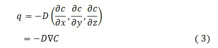
Where, the ∇ is so called gradient operator.
The three-dimensional mass budget is considered when all the mass of the substance must be accounted for:
Rate of accumulation=Σimports-Σexports+Σsource-Σsinks
For an infinitesimal 3D box the volume dxdydz(Figures 2 and 3) the statement becomes:

Figure 2. Flux components in the three-dimensional space.

Figure 3. Flux components in the three-dimensional space.
Where ∇ is the so called divergence operator; with the flux given by diffusion law.
With D taken as a constant, this reduces to:
Where ∇2 is the Laplace operator or Laplacian? It is defined by
Instantaneous localized release without convection: The solution of equation (4) is the product of three prototypical solution with spatial variables x, y and z given by;
 .
.
Is a case of a localized and instantaneous release at locations (x0,y0,z0) and at time t=0 quantity M of a substance?
Spreading: Spreading is identical in all the direction with respect to coordinate’s axes. Since r=√(x2+y2+z2) is the distance and time only.
For isotropic, the size of 3D cloud is given by;
In case of anisotropic medium with turbulence in the vertical direction which differs greatly from that in the horizontal direction because of gravity, we define the three distinct diffusion coefficients as:

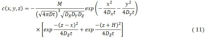
And the solution to an instantaneous (t=0) and localized (x=y=z=0) release

The spatial dimensions of the corresponding 3D cloud are measured by
4σx=4√2DXtIn the x-direction
4σy=4√2DytIn the y-direction
4σz=4√2DztIn the z-direction
Presence of the horizontal boundary
The underground which we take to be flat and horizontal, acts as an impermeable boundary and requires that the vertical component of the diffusive flux be zero at that level (qz=0,t=0)
The solution consist of the sum of two prototypical solution, one caused by the actual release at (x=0,y-0,z=-H)
Where M is the amount released example mass at t=0
The underground concentration
Cground=c(x,y,z=0,t) Where

The ground concentration is highest at the vertical below the release location (x=y=0) and decreases away with distance from there.
Combination of advection and diffusion
When the advective flux is combined with the diffusive flux, then:
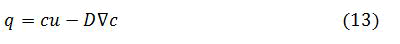
The vector u is the three dimensional vector of fluid medium transporting the substance.
The three dimensional mass budget, by replacement of q by use of (3.11) yield the following equation for the concentration distribution.
We make assumptions that:
• An incompressible medium and compressible effects are negligible.
• The entraining motions must be non-divergent. What converges in one direction must diverge in another. Medium as the uniform diffusion. (constant value of diffusion coefficient D).
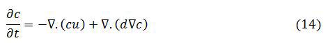
The diffusion-advection equation above become
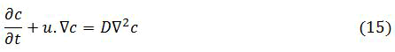
This equation consists of three terms, representing respectively the local accumulation or depletion, the movement by the carrying fluid and the effects of diffusion.
The solution corresponding to instantaneous and localized release in the absence of decay is
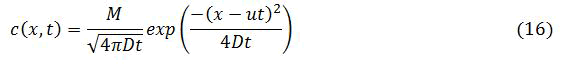
Adding decay and source terms to advection-diffusion equations it become:
The solution corresponding to an instantaneous and localized release is.
Where S=0
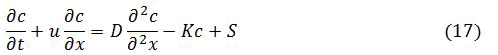
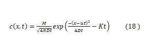
Steady state with advection, diffusion, and decay
In this case, pollutant is continuously discharged at x=0 advected downstream with speed u is diffused in both upstream and downstream direction with diffusivity D, and is continuously withdrawn from carrying fluid at the rate K.
The governing equation is
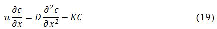
Looking for the solution of the form exp kx with algebraic expression
Introduction
In this chapter, we use set up a suitable environment to carry out a numerical solution of the model equation formulated in chapter three. The solutions of many practical transport problems requires the use of numerical methods because of changes in water saturation (as result of irrigation, evaporation and drainage), spatial and temporal variability of porous properties or complicated boundary or initial condition. Numerical scheme has been a strong tool for analyzing and validating models. It is also helpful in obtaining a numerical solution to a problem which would otherwise be difficult or time consuming obtaining analytic solution. The many numerical methods for solving the ADE can be classified into three groups. Eularian, Langrarian and mixed Langrarian-Eularian methods. In the Eularian approach, the transport equation is discritised by the method of finite difference or finite elements using a fixed mesh. For Langrangian approach, the mesh deforms along with the flow while it is stable in moving coordinates. For mixed approach, the advective transport is solved using a Langrangian approach and the concentration are obtained from particle trajectories. Subsequently all other processes including sinks, sources are modeled using finite elements, finite differences etc.
Numerical solution procedure
There are different numerical techniques by which computer algorithms are derived from equations that govern the model. In order to obtain a numerical model, the mathematical (for example differential) formulation for continuous variables has to be transformed into discrete form. The discrete variables (for example hydraulic head in flow models, concentration, or pressure in transport models) of the model are determined at nodes in the model domain, determined by a grid.
This will entail discretisation procedure of both the aquifer system and the mathematical problems. The discrete equations are such that they apply to the discrete parts of the aquifer. The computer coding, to be presented here also, will solve as many equations as they are for each discrete part of the aquifer. Yet because the discretised parts belong to the same aquifer, what we finally get is the head and reservoir characterization pattern for the entire aquifer.
Stability of the numerical solution
The stability of finite difference method used in the numerical model can be checked by peclet number.
Srinivasan and Mercer suggested that pe<2 and Cr<1 as a guidance for the stability criterion.
Aquifer discretisation
This part is a fundamental aspect of numerical models, which are developed to represent the real world by discrete volumes of material. In numerical modeling, the continuous aquifer domain is replaced by a discretised domain, which consists of an array of nodes and associated finite difference blocks or finite element. Since aquifer properties are assumed to be uniform for each cell, then, the more the cells the greater the ability to vary the hydraulic properties, and reservoir characterization. The modeling area has total of 3884 square kilometres of two dimensional (2D) seismic data covering 8 blocks. The aquifer in this study will be discretised into rectangular cells so as to use the grid set up. In this case, the agricultural field which is a two-dimensional rectangular domain is discretised by a meshgrid of squares and triangles in such a manner that the entire region is covered. Some grids are made fine or course depending on areas of interest and emphasis.
This property makes the calculation of integrals over them less expensive since fewer points of numerical integration are needed than when general quadrangles are used. A total of 3 blocks will be used. This will be representative enough to account for the spatial location of chemo-physical properties and initial conditions of the area. The aquifer exists between depths of 1000 to 3000 meters. In line with this, our aquifer system will be divided into three layers, each measuring 1000 meters thick and will be scaled appropriately. This will total to 100 rows and 100 columns of 888 m × 888 m for each grid block.
Discretisation of the governing equations: Discretisation of the governing equations into discrete components that can be implemented using computer codes will be done to cater for the variation in the chemicals and other agricultural inputs e.g. fertilizer and fungicide etc. physical properties of the aquifer making it possible for an equation to be solved corresponding to each block in the discretized aquifer. This will be discretized using Integrated Finite Difference Method (IFDM). In this method, nodes are centered in the middle of the blocks and flows are assumed to occur perpendicularly to the boundaries of the blocks. Flows between nodes can then be computed using Darcy’s law and the head gradient defined as the difference in heads between neighbouring nodes. With this assumption, a system of equations can be constructed with one equation for each node. This makes it possible to apply the Gauss divergence theorem to the governing equations, converting the integration over block volume to summation over block faces. Applying Gauss’s Divergence theorem on the equations makes it possible to move from volume integral to surface integral. This reduces the order of the P.D.E by one to a first order.
Finite difference approximation of the incompressible fluid flow equation
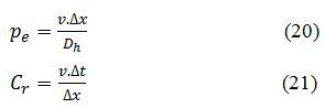
The single phase flow equations derived by use of mass balance equation and Darcy’s equation as described in chapter 3, in i,j,k, components the equation is, in most general form, written in terms of its components as,
Where Δx, Δy and Δz denote the difference along the x,y and z axes respectively and Ax represents the area element normal to the xaxis, and similarly to Ay and Az, while kx, ky and kz are the x,y and z direction permeability and B is the volume element.
This can be simplified to represent incompressible fluid flow in a heterogeneous and anisotropic formulation by use of the following observations.
The density ρ of an incompressible fluid is constant, which implies that viscosity and density bulk volume B is constant, (with B=1 isothermal conditions).
Also, the porous medium is incompressible, which implies that porosity Φ is constant. These assumptions indicate that the right hand side of our equation contains only constants and the temporal derivative vanishes. Setting the partial derivatives with respect to time equal to zero implies that steady state conditions exist.
The resulting equation is:
Where kx=ky=kz=k (constant). For a horizontal reservoir with negligible fluid gravity is constant. Thus equation (4) can be written for every unit volume element as
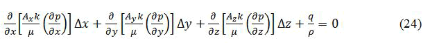
The first step in the process of finding a finite difference solution is to replace equation (5) with its finite difference approximation. The approximation of each partial derivative in equation (5) can be expressed in finite difference approximation as (Figure 4).

Figure 4. Labelling of Grid blocks in the x-y plane.
The coefficients (Axk/μΔx)i+1/2,j,k and similarly in the y and z directions are the transmissibilities, and TΔxi+1/2,j,k and are required at the grid block boundaries.
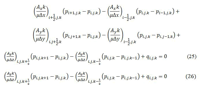
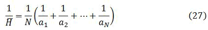
The calculation of these transmissibility are to be calculated individually for each boundary since the dimensions, porosity, thickness, permeability’s etc. of each block may differ. The technique for obtaining averages that we employed is the use of harmonic mean H defined as:
Using the notations above, and assuming homogeinity the entire transmissibility term in the x-direction will be defined as Tx=k/μΔx and the same applies to y and z directions.
Define the transmissibilities at the cell boundaries as follows. Let
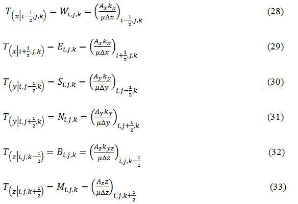
And define the sum of transmissibility’s and the production rate or source term as,
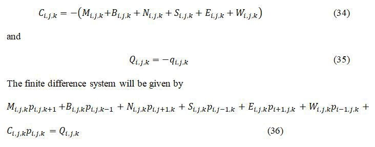
The coefficients defined describe the interaction of the central block to the neighbouring 6 blocks surrounding the central block as shown in Figure 5.

Figure 5. Matrix coefficients for the flow within a cell.
The transmissibility rates specified apply to both cells with wells and those without wells. The wells containing pressure specified wells have the source term qi,j,k unknown (Figure 6).

Figure 6. Downward diffusion of contaminant from the source.
The diagram shows the concentration of contaminants down the cross-section of the region. The concentration at the source point as indicated by the arrow is high which decreases as the depth increases. At the deepest point the concentration of the contaminant is almost zero. The inhabitants residing and using the water from the well will experience health problems since the water from the well will be contaminated as a result of contaminants dissolving in surface water and percolating downwards to the level of the water contained in wells and springs. This shows that inhabitants leaving at the most toxicated area can obtain clean water by maximising the depth of the well as the only option.
Contour concentration and velocity
The contaminants emanating from a localized source such as glysophate in can spread in all directions in the groundwater. Dispersion and diffusion however acts in all three dimensions. The magnitude of the dispersion parameters can vary greatly depending on direction as shown in Figure 7. Region A contains high concentration of glysophate as compared to region B.

Figure 7. Showing contours, concentration and velocity vectors.
The velocity vectors (arrows) indicates how the contaminants spreads from the most toxicated area where many farmers practice mixed farming. The concentration also decreases with increase in the number of contours from the point source. The toxic substance eventually find their way to the nearby streams/rivers causing contamination of water. Inhabitants (both people and animals) residing along these streams/rivers are immensely affected because they depend on these flowing water. Also marine plants and aquatic animals such as planktons fish, frogs, eccetra are greatly affected since the toxic substance can either increase or decrease the ph value of water. Most of them cannot survive in such unfavourable conditions hence destroying the ecological balance.
Decay and sorption in three dimensions
The developed numerical model can be used to describe the effects of non-linearity in the sorption parameters, on time space distribution of the contaminant. Much of the sugar residues are biodegradable matter that undergoes decay and sorption. This retardation factors causes decrease in contaminant concentration with respect to distance from high concentration to a region of low concentration and eventually find their way to the water bodies.
The graph seen below represents the effects of various combinations of decay and sorption to concentration with respect to time and distant. The results shows that release of 100 particles at the source point, the concentration rapidly reduces to 0 at 10, 20 and 30 m with decay, decay and sorption respectively with respect to time and distance (Figures 8 and 9).

Figure 8. Concentration distribution at 1 month.

Figure 9. Concentration Distribution at 240 months.
In this study, particle tracking model has been analyzed. The concentration distribution contaminant is depicted from point source concentration that varies with relative distance away from the source. This concentration gradient causes chemicals from and toxic other farm inputs to diffuse from region of high concentration (A) to a point B. It was realized that the concentration at point A was 2.8 ppm and 0 ppm at point B. Comparatively, the concentration at point A decreases with time and distance away. At point B the concentration increases to approximately 0.6 ppm downstream, 4 kilometers in 10 days. It was noted that point A was the source point with peak concentration mainly glysophate and agricultural inputs. Similarly Figure 6 shows downward diffusion of contaminant from the source point in three dimensions. The concentration at the source point is high and decreases as depth increases. At peak the mass per volume was 0.1 and 0 at 10 meters deep.
The distribution behavior of contaminants is depicted by point source concentration gradient that varies periodically with time against the groundwater flow under realistic boundary conditions and periodic velocity. Because of need of quality water, the government should improve the quality of life through the provision of hygiene sanitation, basic nutrition, and access to clean drinking water. Much research should do on how to neutralize or mitigate the effects of glyphosate and agricultural input areas.
Suggestion for further research
The following areas have been suggested for further research: There is need for research on Particle tracking with difference in the permeability between the three axes.
There is need to research on the effect on contaminant concentration, contuor velocity, decay and sorption with different several random agricultural farms.
[Crossref] [Google Scholar] [PubMed]
[Crossref] [Google Scholar] [PubMed]
Physical Mathematics received 686 citations as per Google Scholar report