Review Article - (2020) Volume 11, Issue 2
Received: 12-Sep-2019
Published:
03-Apr-2020
, DOI: 10.37421/2090-0902.2020.11.315
Citation: Abdelfatah Bouziani, Souad Bensaid and Sofiane Dehilis. “A Second order accurate difference Scheme for the Diffusion Equation with Nonlocal Nonlinear Boundary Conditions.†J Phys Math 11 (2020): 315 doi: 10.37421/JPM.2020.11.315
Copyright: © 2020 Bouziani A, et al. This is an open-access article distributed under the terms of the Creative Commons Attribution License, which permits unrestricted use, distribution, and reproduction in any medium, provided the original author and source are credited.
This paper is considred to solve one-dimensional diffusion equation with nonlinear nonlocal boundary conditions. For the interior part of the problem, our discrete methods use the Forward time centred space (FTCS-NNC), Dufort–Frankel scheme (DFS-NNC), Backward time centred space (BTCS-NNC), Crank-Nicholson method (CNM-NNC), respectively. The integrals in the boundary equations are approximated by the trapezoidal rule. Here nonlinear terms are approximated by Richtmyer’s linearization method. The new algorithm are tested on two problems to show the effciency and accuracy of the schemes.
Forward time centred space with nonlocal nonlinear conditions (FTCS-NNC) • Dufort-Frankel scheme with nonlocal nonlinear conditions (DFS-NNC) • Backward time centred space with nonlocal nonlinear conditions (BTCS-NNC) • Crank-Nicholson method with nonlocal nonlinear conditions (CNM-NNC)
In this paper, we interest to study the numerical solution for the diffusion equation in one-dimensional time-dependent
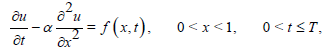 (1)
(1)
with the initial condition
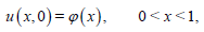 (2)
(2)
and the nonlinear nonlocal boundary conditions
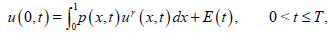 (3)
(3)
 (4)
(4)
Where f,ϕ,p,q,E and G are known functions, so must be determined the function u.
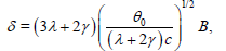
Recently, this kind of nonlocal boundary-value problem with γ=1 has many important applications in chemical diffusion, thermoelasticity, heat conduction processes, population dynamics, vibration problems, nuclear reactor dynamics, biotechnology and mathematical biology, and so forth [1-4] and the references theiren. Also, this problem arises in the quasi-static theory of thermoelasticity treated by several mathematicians such as Day [5,6], who has shown that the entropy per unit volume u(x,t), satisfies:
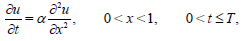 (5)
(5)
 (6)
(6)
 (7)
(7)
 (8)
(8)
where
 (9)
(9)
and
 (10)
(10)
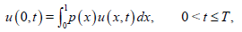
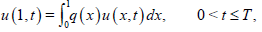
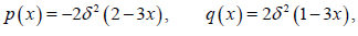
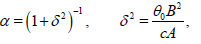
λ and γ are the elastic moduli, θ is the reference temperature, c is the specific diffusion unit volume, and B is the coefficient of the thermal expansion. Dagan [7] describes the quasi-static flexure of a thermoelastic rod of unit length. In this case, the entropy u satisfies (1.5) with the initial condition (1.6) and subject to the nonlocal conditions
 (11)
(11)
 (12)
(12)
where
 (13)
(13)
and
 (14)
(14)
A is the flexural rigidity, the constant B is a measure of the crosscoupling between thermal and mechanical energy and again, θ0 and c denote the reference temperature and specific heat per volume, respectively. The detailed derivation of these equations can be found [8]. Friedman [9] and Kawohl et al. extended the Day’s result which they generalized the parabolic equation in several space variables.
The numerical solution of this problem and its variations has been considered in several papers. Ekolin [10] proved the convergence of the Crank-Nicolson method by using an energy argument, Morton and Mayers [11], and Liu [12] considered the Crank-Nicolson method (θ-method). Fairweather, López-Marcos [13] considered the Crank-Nicolson Galerkin method, Ang [14] solved the problem by using the Laplace transform, Zhi-Zhong Sun [15] used the high order difference scheme and recently, Dehghan [16-18] presented different method explicit and implicit, Martin Vaquero et al. [19,20] presented a new method and discussed this method with Dehghan, Javidi [21] considered the method of lines (MOL), and others [22,23] proposed a general technique for solving the solution in the reproducing kernel space.
In this paper we organized our work as follows:
1. The forward time centred space with nonlinear nonlocal boundary conditions (FTCS-NNBC)
2. The Dufort-Frankel scheme with nonlinear nonlocal boundary conditions (DFS-NNBC)
3. The backward time centred space with nonlinear nonlocal boundary conditions (BTCS-NNBC)
4. The Crank-Nicholson method with nonlinear nonlocal boundary conditions (CNM-NNBC)
5. Numerical experiment
6. Conclusion
Finite difference schemes
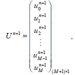
For the numerical solution of the considered problem (1.1)-(1.4) we apply the finite difference technique. First, we take a positive integers N and M We divide the intervals [0,1] and [0,T] into M and N subintervals of equal lengths h = 1/M and k = T/N, respectively. By  we denote the approximation to u at the ith grid-point and nth time step. The Grid point (xi,tn) are given by xi = ih, i = 0,1,2,…,M, tn = nk, n= 0,1,2,…,N.
The notations 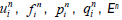 and Gn are used for the finite difference approximations of u(xi,tn), f(xi,tn), p(xi,tn), q(xi,tn), E(tn) and G(tn), respectively.
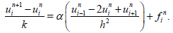
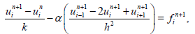
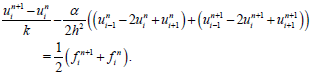
We can approximate the time derivative by the forward difference quotient,and use the second order approximation for the spatial derivative of second order in (1.1) to obtain:
 (15)
(15)
This scheme can be written as:
 (16)
(16)
For i = 1,2,…,M-1, n= 0,1,…,N, and 
Order of accuracy of the scheme is O(k) + O(h2). We still have to determinates two unknowns u0 and uM+1, for this we approximate integrals in (1.3) and (1.4) numerically by trapezoidal rule (We have chosen this approximation since it is of the same, second, order of accuracy in space as the methods used for the interior part of the problem):

 (17)
(17)
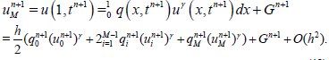 (18)
(18)
Thus, we can write
 (19)
(19)
 (20)
(20)
By applying the Taylor’s expansion
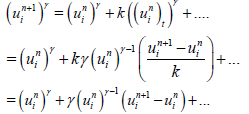
Hence to terms of order k,
 (21)
(21)
a result which replace the non-linear unknown  by approximation linear in
  (the Richtmyer’s linearization method [24]).
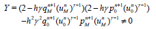
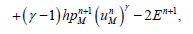
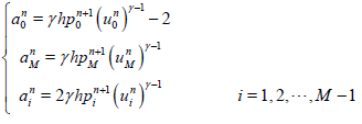
Substituting (2.7) for i=0 and i=M in (2.5) and (2.6), we have
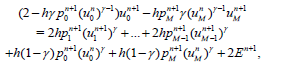 (22)
(22)
 (23)
(23)
Hence we have:
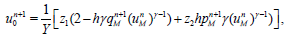 (24)
(24)
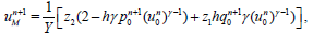 (25)
(25)
where
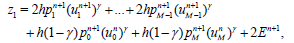 (26)
(26)
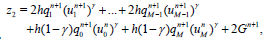
and
 (28)
(28)
(2.14) is true for sufficiently small h.a.
Richardson method is a Central Time Central Space(CTCS) scheme for parabolic type Dufort–Frankel scheme diffusion equations. The application of central differencing for time and space derivative in a straightforward manner to equation (1.1) will yield
 (29)
(29)
This is known as the Richardson method. A stability analysis would show that it is unconditionally unstable, no matter how small k is. Thus, it is of no practical use.
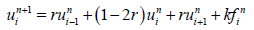
The Richardson method can be modified to produce a stable algorithm. This is achieved by replacing uni on the right-hand side with the time-average of previous and current time values at n-1 and n+1. This new formulation is called Dufort–Frankel scheme and is given by
or
 (30)
(30)
after some rearrangement, we get:
 (31)
(31)
for i = 1,2,...,M-1, n = 0,1,…,N, and r = αk/h2.
Order of accuracy of the scheme is 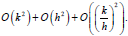 . The scheme is not consistent in the classical sense, but it is if we assume that the ratio
  converge to zero. An optimal choice of k as a function of h to have a high order scheme is to choose k of the same order as h2. In this case, the scheme is of order 2 in space. We still have to determinates two unknowns u0 and um+1 for this we approximate integrals in (1.3) and (1.4) in the same way as in FTCS method.
Note that the Dufort-Frankel method is a two-level method since the stencil contains values of u at two time levels other than the current level n. Consequently, to start the computation, values of u at n and n-1 are required. Therefore, either two sets of initial data must be available or from a practical point of view, a one-step method may be used as a starter to generate additional data. We can use the FTCS method (2.1) with n=0 to find approximate values for uin ,i=1,2,…,M-1 at the first time level, from the known values u0i . Then (3.3) with n=2,…,N, is used to compute approximations to u(xi,tn) This scheme is explicit and can be shown to be unconditionally stable by the von Neumann stability analysis.
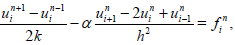
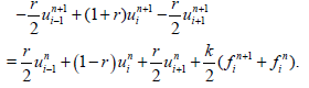
Using the the classical backward time centred space finite difference scheme to approximate the derivative in eqution (1.1), we get
 (32)
(32)
and after some rearrangement, the equation (3.1) becomes
 (33)
(33)
for i = 1,2,…,M,-1, n = 0,1,…,N, and r = αk/h2.
Order of accuracy of this scheme is O(k) + O(h2)
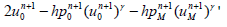
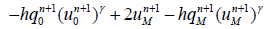
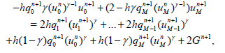
There are M-1 linear equations from (2.4) in M+1 unknowns u0,u1,… um. In order to solve for unknowns, we need two more equations. So, let us formally approximate integrals in (1.3) and (1.4) numerically by the trapezoidal numerical integration rule (the BTCS scheme is second-order accurate with respect to the space variable) :
 (34)
(34)
 (35)
(35)
By applying the Richtmyer’s linearization method (2.7) in (4.3) and (4.4), we have
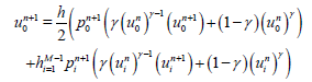 (36)
(36)
 (37)
(37)
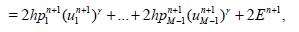
Thus, we can write (4.5) and (4.6) as follows
 (38)
(38)
 (39)
(39)
 (40)
(40)
where
 (41)
(41)
and
 (42)
(42)
and also
 (43)
(43)
where
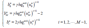 (44)
(44)
and
 (45)
(45)
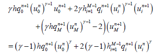
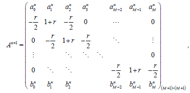
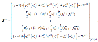
Combining (4.10), (4.13), with (4.2) yields an (M+1) × (M+1) linear system of equations. We write the system in the matrix form
 (46)
(46)
which
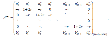 (47)
(47)
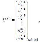 (48)
(48)
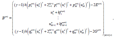 (49)
(49)
where  are the coefficients in (4.10) and (4.13), respectively.
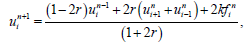
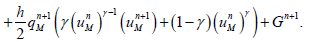
Theorem 1: The BTCS scheme has a unique solution for sufficiently small h.
Proof. It is easy to see that |1 + 2 -r |>|2r|, the matrix (4.16) is diagonally dominant (thus it is non singular), if
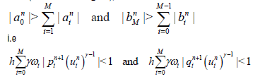 (50)
(50)
Where ω0=ωm=1/2, ωi=1, i=1,…,M-1. As (4.19) is true for sufficiently small h, the existence and uniqueness of the solution of BTCS scheme are proved.
The Crank-Nicholson Method with Nonlinear Nonlocal Boundary Conditions (CNM-NNBC)
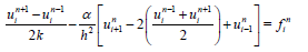
To get abetter approximation for  , we give the Crank-Nicholson scheme to approximate equation (1.1), then we have :
 (51)
(51)
and after some rearrangement, the equation (1.1) becomes
 (52)
(52)
for i = 1,2,…,M-1, n = 0,1,…,N, and r = αk/h2.
Order of accuracy of the scheme is O(k2) + O(h2)
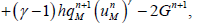
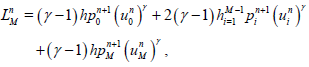
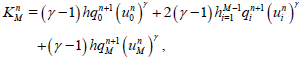
Crank-Nicholson finite difference technique is second-order accurate with respect to the space variable, so the integrals in the boundary conditions (1.3) and (1.4) will be approximated in the same way as in the BTCS method. Combining (4.10), (4.13), with (5.2) yields an (M+1) × (M+1) linear system of equations. We write the system in the matrix form
 (53)
(53)
which
 (54)
(54)
 (55)
(55)
 (56)
(56)
where  are the coefficients in (4.10) and (4.13), respectively.
Theorem 2 The CNM scheme has a unique solution for sufficiently small h.
Proof. It is easy to see that |1+r|>|r| the rest is obtained by following the same procedure done in establishing the proof of theorem 1.
Numerical experiments
To test the above algorithms described in Section 2-5, we use two examples with known analytical solutions as follows:
Example 1: We consider the following problem (Test given in paper [25] they used a fourth-order accurate difference scheme [26-28])
 (57)
(57)
subject to the initial condition
 (58)
(58)
and the nonlinear nonlocal boundary conditions
 (59)
(59)
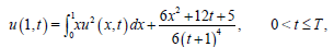 (60)
(60)
The functions f,ϕ,p,q,G and E are chosen so that the function
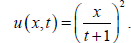 (61)
(61)
is the exact solution solution of the problem(1.1)-(1.4)
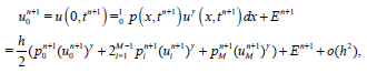
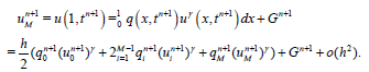
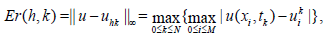
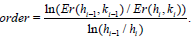
In Tables 1 and 2 we present results with h=0.05, 0.005 and r=0.4 using the finite difference formulate discussed in section 2-5 together with the results from [2] for x=0.1 and t=0.01, 0.02, 0.03,…0.1.. Table 3 and Table 4 gives the maximum errors of the numerical solutions experimental order of convergence. The maximum error is defined as follows
| ti | exact | FTCS | DFS | BTCS | CNM | results from [2] |
|---|---|---|---|---|---|---|
| .01 | 0.0098029 | 0.0103508 | 0.0103390 | 0.0103547 | 0.0103523 | 0.0093 |
| .02 | 0.0096116 | 0.0103461 | 0.0103425 | 0.0103573 | 0.0103515 | 0.0091 |
| .03 | 0.0094259 | 0.0102447 | 0.0102440 | 0.0102646 | 0.0102545 | 0.0090 |
| ... | ... | ... | ... | ... | ... | ... |
| .1 | 0.0082644 | 0.0091799 | 0.0091850 | 0.0092375 | 0.0092086 | 0.0079 |
| ti | exact | FTCS | DFS | BTCS | CNM | results from [2] |
|---|---|---|---|---|---|---|
| .01 | 0.0098029 | 0.0098085 | 0.0098085 | 0.0098086 | 0.0098085 | 0.0098 |
| .02 | 0.0096116 | 0.00961190 | 0.0096190 | 0.0096192 | 0.0096191 | 0.0096 |
| .03 | 0.0094259 | 0.0094341 | 0.0094341 | 0.0094343 | 0.0094342 | 0.0094 |
| ... | ... | ... | ... | ... | ... | ... |
| .1 | 0.0082644 | 0.0082736 | 0.0082736 | 0.0082742 | 0.0082739 | 0.0083 |
| M | N | FTCS | order | BTCS | order |
|---|---|---|---|---|---|
| 40 | 2.4·10-3 | 2.99×10⁻³ | |||
| 160 | 6.08·10-4 | 1.984 | 7.41·10-4 | 2.015 | |
| 640 | 1.52·10-4 | 1.995 | 1.84·10-4 | 2.004 | |
| 2560 | 3.81·10-5 | 1.998 | 4.62·10-5 | 1.999 |
| M | N | CNM | order | M | N | DFS | order |
|---|---|---|---|---|---|---|---|
| 40 | 2.68·10-3 | 4 | 16 | 1.77·10-3 | |||
| 80 | 6.70·10-4 | 2.003 | 8 | 64 | 4.51·10-4 | 1.971 | |
| 160 | 1.67·10-4 | 2.000 | 16 | 256 | 1.130·10-4 | 1.996 | |
| 320 | 4.18·10-5 | 2.000 | 32 | 1024 | 2.82·10-5 | 1.999 |
and the experiment order convergence is calculated using the formula :
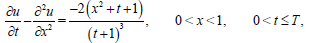
Example 2: The second test example to be solved is
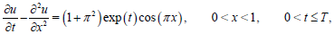 (62)
(62)
with the initial condition
 (63)
(63)
and the nonlinear nonlocal boundary conditions
 (64)
(64)
 (65)
(65)
The analytic solution is
 (66)
(66)
In Tables 5 and 6 we present results with h=0.05, 0.005 and r=0.4 using the finite difference formulate discussed in section 2-5 for x=0.1 and t=0.01, 0.02, 0.03,…, 0.1. Table 7 gives the amount of CPU-time used, in seconds, for the computation on an Intel Core i3 with 2.1 GHz computer.
| ti | exact | DFS | FTCS | BTCS | CNM |
|---|---|---|---|---|---|
| .01 | 0.96061479 | 0.96074288 | 0.96074308 | 0.96074404 | 0.96074352 |
| .02 | 0.97026913 | 0.97046058 | 0.97046112 | 0.97046570 | 0.97046320 |
| .03 | 0.98002050 | 0.98025235 | 0.98025315 | 0.98026012 | 0.98025629 |
| ... | ... | ... | ... | ... | ... |
| .1 | 1.05108000 | 1.05140348 | 1.05140505 | 1.05141906 | 1.05141129 |
| ti | exact | FTCS | DFS | BTCS | CNM |
|---|---|---|---|---|---|
| .01 | 0.96061479 | 0.96061606 | 0.96061606 | 0.96061612 | 0.96061609 |
| .02 | 0.97026913 | 0.97027103 | 0.97027104 | 0.97027113 | 0.97027108 |
| .03 | 0.98002050 | 0.98002280 | 0.98002282 | 0.98002892 | 098002286 |
| ... | ... | ... | ... | ... | ... |
| .1 | 1.05108000 | 1.05108323 | 1.05108325 | 1.05108340 | 1.05108331 |
| M | N | FTCS | DFS | BTCS | CNM |
|---|---|---|---|---|---|
| 160 | 1.59 | 2.12 | 2.13 | 2.25 | |
| 640 | 22.69 | 23.34 | 29.22 | 30.14 | |
| 2560 | 204.50 | 209.26 | 274.65 | 284.34 | |
| 10240 | 1423.03 | 1532.45 | 2986.06 | 3194.61 |
In this paper new techniques were applied to the one-dimensional diffusion equation with nonlinear nonlocal boundary conditions. The numerical results obtained by using the methods described in this article give acceptable results and suggests convergence to the exact solution when h goes to zero. The FTCS method is explicit and require less computational time than the other implicit schemes (Table 7), but the disadvantage of this discretization is the strict stability criterion  . The finite difference techniques proposed in this paper can easily be extended to the similar two and multi-dimensional problems.
Physical Mathematics received 686 citations as per Google Scholar report