A Lattice Model of COVID-19 Epidemic

George R Gavalas^*
*Correspondence: Dr. George R Gavalas, Department of Chemistry and Chemical Engineering, California Institute of Technology, Pasadena, California, USA, Email:

Keywords

COVID-19 • Lattice model • Computer simulation

Introduction

Epidemic disease models have been developed by epidemiologists, statisticians, physicists and others. The models developed over the years can be classified in several broad classes: (i) branching process models, (ii) differential equation models, (iii) network models. (iv) statistical models that describe disease progress by some analytical function containing parameters to be determined from data by statistical estimation. Models (iv) are purely empirical and do not provide a basis for planning mid-term intervention. Type (i) models utilize branching process theory and have been applied by epidemiologists to actual data from measles and other epidemics [1-3]. They are relatively simple and can draw on exact results from probability theory. Differential equation models (ii) are very popular because systems of ordinary differential equations can be readily formulated and can be readily solved numerically, or even analytically, in highly simplified form. Examples include the early paper of Kermack and Kendric, and the recent paper of Poletti that includes a behavioral element in the equations [4,5]. The type (ii) models imply complete mixing or homogenization of all individuals and have also been labelled mass action models. The basic theory for these models is treated in Bailey’s well known book [6]. Network models (iii) have been developed using methodology of Statistical Physics. They employ nodes of susceptible, infective and other individuals interconnected in a network or graph. Using sophisticated statistical averaging network models lead in some limiting cases to analytical results [7,8]. A recent paper by Volz combines elements from network and differential equation models [9].

In this paper we present a model in which individuals are located on a lattice, where each individual occupies a lattice cell and is labeled by the cell coordinates. Individuals are allowed to interact with neighboring or furtherlocated individuals on a probabilistic basis. There is no homogenization. The model is flexible but does not lend itself to analytical results. It entails purely computer simulation. The lattice model is defined in section 1. Section 2 discusses the significance of model parameters and presents sample results of simulations. Section 3 summarizes conclusions. The computer code was written in Python.

Literature Review

Model description

The lattice: A n × n square lattice is defined where each cell contains one individual of a particular type, or is vacant. Each individual is labelled by its cell coordinates (i,j) and by an index defining its type (susceptible, infective e.t.c.). Of the n² cells the 4n-4 cells belonging to the lattice edges are not occupied in order to simplify the code. Hence, the total number of individuals on a n × n lattice is n²-4n+4.

The individual types: The following types of individuals are recognized.

Type 1: healthy and mobile, susceptible to infection, briefly labelled “susceptibles”.

Type 2: healthy and immobile, not susceptible to infection.

Type 3: dead.

Type 4: recovered from disease and assumed immune to further infection.

Type 5+q: mobile infected. These individuals can infect type 1 individuals and are referred to as “infectives”. There are k1 types of infectives, labelled 5+q, where q=0,…,k1-1. These types are assumed asymptomatic or mildly sick. A freshly infected individual carries index 5. The increment q is the number of days since infection. When infected a type 1 individual is converted to type 5. Upon reaching age q=k1 an infective is converted to recovered, type 4, with probability p4, otherwise progresses to type 5+q, q=k1,…,k1+k2.

Type 5+q, q=k1,…,k1+k2: These individuals are assumed hospitalized and isolated. They are assumed not to be infective. Upon reaching age k1+k2 an individual of this type either recovers to type 4 with probability p5, or dies with probability 1-p5.

The initial conditions: Initially the lattice is populated with individuals of type 1, a small number of type 5, or are left vacant. The vacant cells remain unoccupied throughout the simulation.

Mobility and infection: Disease progression proceeds in discrete time increments of one or more days each. At each discrete time all n2-4n+4 cells are quarried one by one. Each type 1 encountered (susceptible) is allowed with probability p1 to convert to type 2. If not converted to type 2 it is allowed to move in one of the following four directions: increasing j, decreasing j, increasing I, decreasing I, all with equal probability determined by a random integer generator. Once a direction is selected, the feasible length h of the movement (in cell units) is selected by a random integer generator within the range allowed by the lattice boundary. Then a function f(h) is defined that renders longer lengths less likely:

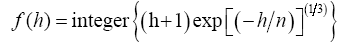
where “int” denotes the integer value of the number. A movement of length f(h) (in cell units) is then implemented. If the individual at the cell reached is infective (5+q, q=0,…k1-1), the cell at (i,j) is converted to type 5. If the cell reached by the movement is of any other type, the individual at (i,j) does not change. Whether infected or not, the type 1 individual after the move is returned to its original cell (i,j). It is noted that the step size f(h) defined above increases with the lattice size n, but less than proportionately.

Each infective individual (type 5+q, q=0,…,k1-1) that is reached in the scan is allowed to move by exactly the same rules as for type 1 above. If the move leads to a type 1 individual, the latter is converted to type 5 with probability p3. The infective individual is returned to its initial position (I,j). At each time step the infective individual’s index is increased from 5+q to 5+q+1. Upon reaching 5+k1, the infective is either converted to type 4 (recovered) with probability p4 or becomes hospitalized or isolated (type 5+q, q=k1,…,k1+k2-1). For the latter type of individuals, q is increased by unity at each time increment. Upon reaching 5+k1+k2 the individuals of this last type either recover with probability p5 or die with probability 1-p5. As a result of these rules after k1 days the infectives are either recovered or hospitalized. The hospitalized individuals are assumed not to be infective due to strict hospital precautions.

Significance of parameters and sample results

Initial number of type5 (Infectives): The following runs employ the parameters in Table 1 except as indicated.

Each run constitutes a discrete stochastic process controlled by probabilities p1,p3,p4,p5 set at the beginning of the run. The probabilities are implemented by random numbers from a uniform distribution in (0,1). The sequence of random numbers during execution is generated by a Random Number Generator (RNG) using some specified “seed”. Each time the same seed is used the same random number sequence is generated. The seed for each run is specified by the user or is generated by the RNG.

Three sets of 16 run each were carried out using different seeds for each run. The parameters of Table 1 were used with p3=0.04 and a single initial infective (type5) at grid position (25,25). The results are summarized in Table 2 which lists for each set the mean and standard deviation (sdv) of dead and recovered at the end of the infection. The end is defined by the disappearance of the last type5 (infective). In the 48 runs the number of dead varied from 0 to 33 and the recovered from 47 to 491. Most of the runs had zero dead while a few had a relatively large number. The time evolution of the infection for two runs, one with zeros dead the other with a relatively large number of dead. The number of recovered also exhibits large variability. These results imply that the course of infection caused by a single infective in a population of approximately 2500 will be unpredictable.

Two sets of runs were next carried out using the parameters of Table 1 with p3=0.04, but with 10 initial infectives randomly distributed over the lattice. The rest of the cells were all initially occupied by type1. The means and sdv’s of these runs are also included in Table 2. The sdv’s are still large but the relative sdv’s are considerably lower than in the single infective sets. The duration of infection is longer, 150-300 days versus 30-150 for the first three sets. Samples out of the two sets starting with 10 infectives. A useful measure for comparison with public health data is the ratio of recovered to dead at the end of the infection. This ratio varies between 14 and 40 throughout Table 2 (Tables 1 and 2).

Lattice size

To examine the effect of lattice size, i.e., population, two sets of 16 runs were conducted using parameters from Table 1 but for an 100 × 100 lattice (9,604 cells) and for 10 or 40 initial infectives. As before the runs in each set differ only by the random sequence used. The results are presented in Table 3 which also includes a set from the 50 × 50 lattice for comparison. The first two columns show similar high variability in both dead and recovered. In the last column obtained using 40 initial infectives variability has sharply diminished while the mean of dead has increased roughly by a factor of 4. The ratio of recovered to dead is 15-17 throughout the three sets (Table 3).

Density

In the runs so far all cells were initially occupied by type1 or type5. To explore the effect of lower number of occupied cells, i.e., lower population density, runs were carried out using the parameters of Table 1 with a fraction f of unoccupied cells randomly distributed throughout the lattice. Some results are shown in Table 4 for f=0, 0.2, 0.4. The number of dead and recovered decrease roughly by a factor of 3 from f=0 to f=0.2, and by another factor of 3 from f=0.2 to f=0.4. At f=0.4 the number of dead shows increased uncertainty. The numbers of recovered show larger regularity for all three values of f (Table 4).

The parameters p3 and k1 have the largest effect on the duration infection and the total number of dead and recovered. In all simulations up to this point p3 was set at 0.04. Runs were next performed using p3=0.03 and p3=0.05, with the other parameters from Table 1. The results are summarized in Table 5. Each of the three columns summarizes 16 runs differing only by the random sequence employed. At p3=0.03, k1=15 the numbers of dead and recovered are low and show large uncertainty. At p3=0.04, k1=15, a case already included in Table 2, the numbers of dead and recovered increase sharply but the large uncertainty remains. At p3=0.05 the number of dead and recovered increases further sharply and the uncertainty decreases sharply. Comparison of the results in the third and 5th column with the standard case in column 2 shows that increasing p3 or k1 results in similar large increase in the number of dead and recovered. The duration of infection increases from left to right but is less variable than the number of dead. The other two parameters p4 and k2 can in principle be estimated from clinical observations. We have used p4=0.8 as the probability that an infected individual recovers and does not get admitted to the hospital. Increasing p8 would reduce the number of infectives and increase the number of recovered reducing the duration of infection and the number of dead. The last parameter k2 has no effect on the number of cases (infections) and only influences the relative number of dead and recovered. It can be directly obtained from hospital data (Table 5).

Length of movement

The interaction distance between susceptibles and infectives at each time step was so far determined according to the “standard rule”, defined in the section “Model Description”. A simpler alternative is to employ a step of fixed length subject to the geometric constraints of the lattice boundary. For this purpose a distance z is chosen randomly among the available distances to the boundary. The step length is then defined as the minimum between z and some preassigned number nmax. Table 6 summarizes results for the 50 × 50 lattice for 3 values of n max. As in the previous tables each set involves 16 runs differing only by the random sequence used. The table also includes a set labelled “standard rule” from previous tables. The numbers of dead, recovered, and the duration increase with increasing nmax since more susceptibles become accessible as infection progresses. The results using the “standard rule” are relatively close to nmax=20 (Table 6).

Intervention

The probability p1 of conversion of Type1 (susceptible) to type 2 (isolated) at each time step was kept zero in all runs up to this point. Positive values of p1 would clearly slow the infection. A simple way of using p1 as a tool for intervention is to start with p1=0, and switch to some p1>0 when the number of cases per day exceeds a predetermined value b. The results of this very simple feedback mechanism are given in Table 7 for p3=0.05, 10 initial infective, with the other parameters from Table 1. The first 16-run set is for p1=0 (earlier result from Table 5), the other columns for different sets of p1 and b.

With the low probability p1=0.005 but low b=5, already the number of dead and recovered is sharply reduced from the base case p1=0. With the probability p1 increased to 0.01 the number of dead and recovered is further decreased to p1 approximately 25% of the base case. At p1=0.01 but at higher trigger b=10 the number of dead and recovered approximately doubles from the lows. The higher trigger delays the intervention. Of the two parameters p1 and b, the second appears more practical to implement (Table 7).

Discussion

A major feature of the model is the introduction of age q as an index of infectives (number of days since infection). This feature permits controlled recovery of infectives which is the main mechanism of epidemic termination.

The model contains parameters p1, p4, p5, k1, k2 that have an obvious interpretation and can be roughly estimated from published reports. It is assumed throughout that the infectives either recover or become hospitalized or isolated becoming non-infective. Among the various probabilities, p3 cannot be directly obtained from measurements but must be estimated by matching model predictions to reported number of cases, dead, and recovered. This matching would have to consider that the parameters p3 and k1 are strongly correlated.

A major conclusion of the simulations is the high degree of uncertainty in the results of each run, as they depend on the particular sequence of random numbers used. To compare the effect of different sets of parameters, mean and standard deviation (sdv) were obtained for 16 runs for each set. In some cases, especially for low values of p3, the standard deviation is on the same order of magnitude as the mean. Using a larger lattice, i.e., a larger population would reduce the uncertainty but the required increase the computational effort is beyond the scope of the study. Hence, simulations were carried out for only 50 × 50 and 100 × 100 lattices.

Conclusion

The model explores the effect of population density and distance travelled by susceptible and infective individuals. It also evaluates the effectiveness of isolating a fraction of susceptibles during the pandemic when the number of daily cases exceeds a specified number.

A major weakness of the model is treating the population as discrete individuals. Families or clusters of individuals in close contact are not considered although current reports suggest that a single infective can cause infection to several individuals in close proximity. The model also treats an isolated population with interaction between neighboring populations neglected. At this time data from isolated communities of the right size were not available to test the model. It is only noted that the ratio of recovered to dead, 15-40 in Tables 2 and 3 is in the range reported for a number of US states or counties.

References

1. Farrington, Paddy, Mona Kanaan and NJ Gay. “Branching Process Models For Surveillance of Infectious Diseases Controlled By Mass Vaccination.” Biostatistics 4(2003): 279-295.

   [Crossref] [Google Scholar]

2. Blumberg, Seth, Sebastian Funk and Juliet Pulliam. “Detecting Differential Transmissibilities That Affect the Size of Self-Limited Outbreaks.” PLoS Pathog 10(2004): 1004452.

   [Crossref] [Google Scholar]

3. Nishiura, Hiroshi, Kenji Mizumoto and Yusuke Asai. “Assessing the Transmission Dynamics of Measles in Japan, 2016.” Epidemics 20(2017): 67-72.

   [Crossref] [Google Scholar]

4. Kermack, William Ogilvy and McKendrick. “A Contribution to The Mathematical Theory Of Epidemics.” Proc R Soc Lond 118(1927): 700-721.

   [Crossref] [Google Scholar]

5. Poletti, Piero, Marco Ajelli and Stefano Merler. “Risk Perception And Effectiveness Of Uncoordinated Behavioral Responses In An Emerging Epidemic.” Math Biosci 238(2012): 80-89.

   [Crossref] [Google Scholar]

6. Bailey Norman. “The Mathematical Theory Of Infectious Diseases and Its Applications.” Hafner Press, New York 72(1975): 475-488.

   [Google Scholar]

7. Newman Mark. “Spread of Epidemic Disease On Networks.” Phys Rev E 66(2002): 016128.

   [Crossref] [Google Scholar]

8. Satorras, Romualdo Pastor, Alexei Vázquez and Alessandro Vespignani. “Dynamical and Correlation Properties of the Internet.” Phys Rev Lettrs 14(2001): 258701.

   [Crossref] [Google Scholar]

9. Volz, Erik and Lauren Ancel Meyers. “Susceptible–Infected–Recovered Epidemics in Dynamic Contact Networks.” Proc R Soc B 274(2007): 2925-2933.

   [Crossref] [Google Scholar]