Research Article - (2022) Volume 13, Issue 11
Received: 01-Aug-2022, Manuscript No. BEJ-22-70854;
Editor assigned: 04-Aug-2022, Pre QC No. BEJ-22-70854(PQ);
Reviewed: 19-Aug-2022, QC No. BEJ-22-70854;
Revised: 30-Sep-2022, Manuscript No. BEJ-22-70854(R);
Published:
08-Oct-2022
, DOI: 10.37421/2151-6219.2022.13.411
Citation: Skander, Ben Hassine, and Aouadi Sami. "Foreign
Direct Investment, Institutions and Economic Growth." Bus Econ J 13 (2022):
411.
Copyright: © 2022 Skander BH, et al. This is an open-access article distributed under the terms of the creative commons attribution license which permits
unrestricted use, distribution and reproduction in any medium, provided the original author and source are credited.
The importance of a favorable climate in determining FDI flows has been understood and emphasized in the economic literature for a long time. Thus, the inclusion of various measures of social and political attributes of host countries is not an aspect of recent literature for FDI. We can cite the studies of Basi who investigated the effects of political instability on FDI. However, in recent years there has been a resurgence of interest in this subject, with particular emphasis on the factors representative of the quality of institutions. A huge number of papers that address this will lead to a burgeoning literature on the effect of FDI on economic growth via the quality of institutions. Three factors contributed to the emergence of this interest. First, in North study, there has been widespread awareness of the important role played by institutions in shaping incentives for investment and economic activities in general. Second, there was a rapid growth in FDI flows in the 1990, and the growing interest of transition and developing countries in attracting a larger share of these flows. Third, foreign investors have shown a greater interest in the quality of institutions over access to conventional natural resources and view it as a potential location advantage in host countries.
The purpose of our research is to try to explain theoretically and empirically how and to what extent the quality of institutions conditions the impact of Foreign Direct Investment (FDI) on economic growth? and this with the aim of drawing lessons for possible economic policies.
The two panel data models involve a sample of 110 countries, further divided into two groups: 40 PD and 70 PVD, using GMM system, our results show that FDI alone plays an ambiguous role in contributing to economic growth during the period from 1996 to 2017.
FDI • GDP • Institutions • JEL classification
The question of whether Foreign Direct Investment (FDI) contributes to enhancing economic growth has been one of the fundamental questions in international economics and development, and has received much attention in the economic literature in recent years.
However, it seems that this question is not yet resolved. Given recent developments in economic growth theory, which emphasize the importance of improving technology, factor efficiency and productivity in determining economic growth, FDI can have a positive impact on growth [1]. FDI, seen as a mixture of capital, know-how and technology, can increase the level of existing technology in host countries in several ways [2].
However, given the available empirical evidence, it is difficult to conclude that there is a universal relationship between FDI and economic growth [3]. Empirical evidence has shown that FDI can have positive, negative or negligible effects on economic growth [4].
More recently, some empirical studies have shown that all host countries are capable of reaping the positive externalities offered by FDI, and that the positive impact of FDI on economic growth essentially depends on the absorptive capacity of host countries. The term “absorptive capacity” limit includes such factors as the degree of quality of institutions, levels of financial development, level of economic development, etc. Several empirical studies prove that the economies of host countries must reach a certain level of absorptive capacity, called the development threshold, to be able to benefit from FDI.
We wish to present in this article a general overview of the effects of FDI on economic growth, taking into account the role of the quality of institutions in the host countries. This chapter is organized as follows: Section one, provides an overview of the impact of FDI on economic growth. Section two presents an empirical test using the GMM method and discusses the importance of the quality of institutions from this perspective.
Traditional analyzes around the impact of FDI on economic growth and its classic effects.
The impact of FDI on economic growth: Economic theory attributes an important role of FDI on economic growth in developing countries because, on the one hand, new theories of economic growth emphasize the crucial role of technological progress and the creation of new ideas in determining the growth rate, and on the other hand, the literature indicates that FDI is one of the most important channels through which technologies can be transferred to developing countries, then FDI plays this role because multinational firms have technological advantages to local firms [5-7].
The theory of exogenous growth and FDI: Exogenous growth theory, commonly known as neoclassical growth theory, was pioneered by Solow. This theory assumes that economic growth is generated by exogenous factors in the production function such as the accumulation of capital stock and labor.
Barro and Sala-i-Martin demonstrate that there is a positive relationship between economic growth and capital accumulation over time.
According to this theory, an increase in the stock of capital accumulation will result in an increase in growth assuming that the quantity of labor and the level of technology remain constant [8]. So on the one hand, economic growth is determined by the stock of capital accumulation, the rate of savings and the rate of depreciation of capital. On the other hand, economic growth is determined by exogenous factors such as technical progress which takes the form of an increase in the labor force in the long run [9].
Thus, the growth of the economy depends on the stock of capital accumulation and the increase in the labor force as technical progress. In this sense, the news technology introduced by FDI leads to an increase in labour, capital accumulation and productivity which will lead to more regular returns to investment if labor will grow exogenously [10]. In general, this theory holds that FDI increases the stock of capital in the host country, and then promotes economic growth towards a new equilibrium state through this accumulation of capital. The argument of exogenous growth theory is that FDI affects short-term economic growth through diminishing returns to capital; therefore FDI promotes economic growth through increased Domestic Investment (DI) [11].
An abundant economic literature indicates that FDI, as a combination of the stock of capital, technology and management experience and entrepreneurial abilities, can affect economic growth in two distinct ways. On the one hand, FDI represents a new addition to the capital stock of host countries, and therefore can contribute positively to economic growth. However, in the standard neoclassical growth model, the contribution of FDI to economic growth as capital accumulation is limited, due to diminishing returns to capital [12]. In other words, according to the neoclassical growth model, the impact of FDI on economic growth is similar to the impact of domestic investment, in that it is a transitory impact and has no bearing on the long-term economic growth rate [13]. Long-term economic growth is affected only by technical progress and the growth rate of the working population, all of which are considered exogenous according to the neoclassical growth model [14].
The main limitation of this theory is considering human capital (knowledge) as work. Economically, knowledge is human capital because knowledge is accumulated and stored in business systems. In addition, this theory does not sufficiently explain the production, diffusion of technology and knowledge because the information gradually becomes evident in economic analysis [15]. Also this theory does not provide the long-term explanation of economic growth and technical progress [16].
Endogenous growth theory and FDI: In the mid-1980, exogenous growth theory became theoretically insufficient to explain the determinants of long-term growth [17]. Therefore, endogenous growth theory was launched by Romer in his paper in 1986, which is focused on two factors human capital and technical progress.
Economic growth is derived by the stock of human capital and then by technological developments [18]. The mechanism of this theory regarding the stock of human capital is that labor grows as a share of the population. This means that growth is favored exogenously at a constant rate. Subsequently, this growth is stimulated by a multiplier that increases both technology and labor, which means that this growth is promoted endogenously by the increase in labor and technological change [19].
However, the main feature of this theory is the absence of diminishing returns to capital [20]. Therefore, technological progress in the form of new idea generation is a crucial factor in diminishing the diminishing return to capital over the long term. The theory holds that technical progress is endogenously enhanced by taking for example knowledge from Research and Development (R and D) and that the development of this knowledge can create positive externalities and positive spillovers on growth [21]. As a result, R and D, human capital accumulation and spillovers are seen as the main determinants of long-term economic growth [22]. The effects of knowledge generated by R and D in one country create positive effects in other countries [23]. Endogenous growth theory identifies economic growth as fostered in the long run by the introduction of new technologies into the production process in host countries, and that FDI is assumed to be more productive than FDI [24]. Thus, FDI promotes economic growth through technological surpluses. These offset the effects of diminishing returns to capital by stimulating the current stock of knowledge through labor mobility, training, skills and through managerial qualification and organizational arrangements [25]. Moreover, FDI should strengthen the existing stock of knowledge in the recipient economy, through the formation of manpower and the acquisition of skills and the diffusion of technology; and also through the introduction of alternative management practices and organizational arrangements. Generally speaking, the existence of various forms of externalities prevent the unbridled decline of the marginal productivity of capital. As a result, foreign investors can increase the productivity of the host economy and then FDI can be seen as a driver of FDI and technological progress. Furthermore, the mechanism by which FDI promotes growth in the host country should be a large potential for the externality effect of FDI [26]. Thus, economic growth can increase indefinitely over time via FDI [27].
In endogenous growth models, on the other hand, FDI is seen as a catalyst for productivity improvement and technological progress, and thus it has a long-term effect on economic growth [28]. In these models, FDI has an effect on endogenous economic growth, as it creates increasing returns to capital through positive externalities of technology [29]. In general, it can be said that the economic literature indicates that the contribution of FDI to economic growth comes not only through its contribution to capital accumulation, but also through its role as a vehicle for knowledge transfer and new technologies and other management experiences, all of which are expected to increase the level of productivity and leading to higher rates of economic growth in the host countries. Technology can be transferred through several channels, including international trade. However, FDI and the activities of Multinational Enterprises (MNEs) in host countries represent the main channels through which technology diffusion can take place. This is because multinational companies conduct most of the Research and Development (R and D) in the world and therefore they are among the companies that acquire the most advanced technology in the world. Moreover, FDI not only provides the host economy with advanced technology, but also with the necessary complements of these technologies, such as managerial experience and entrepreneurial abilities.
Although, the biggest limitation of this theory is that its invalid predictive ability on growth convergence to account for the heterogeneity of economies and their different growth patterns, FDI can promote economic growth in several ways.
Some researchers argue that the effects of FDI on economic growth are believed to be two- fold. First, FDI can affect economic growth through capital accumulation by introducing new foreign goods and technologies. This view comes from exogenous growth theory. Second, FDI can stimulate economic growth by expanding the stock of knowledge in host countries through knowledge transfer.
This view comes from endogenous growth theory. Theoretically FDI can play a crucial role in economic growth by boosting capital accumulation and technical progress.
Figure 1 shows the circular flow of dynamic relationships between FDI, FDI and economic growth and the direct and indirect effects of FDI flows on economic growth. In this figure as can be seen, through three channels FDI can affect economic growth:
• FDI can affect economic growth directly as an investment channel (I).
• FDI can affect economic growth indirectly through influence on DI (III*+II*, attraction effect).
• FDI can also affect economic growth indirectly through technological improvement in host countries by generating positive externalities (III+IV*, spillover effect) or crowding out FDI through linkage effect (III+IV+IV*).
In fact, the figure also shows the causal link between FDI, ID and economic growth. The channel (I+I*) demonstrates the causal relationship between FDI and economic growth.
Also, the channel (II**+II*) illustrates the dynamic relationship between DI and economic growth. The causal relationship between IDE and DI can also appear in the channel (III*+III**).

Figure 1. The circular flow of the dynamic relationship between FDI, DI and GDP.
The impact of FDI on economic growth: Empirical studies based on all the assumptions. And quite recently, using both the twostage least squares (DMC) method and the GMM method, in an econometric study on a panel of 65 developing countries over the period from 1985 to 2015, puts highlight the role of human capital as a determining factor in the transmission of technologies and productivity gains via FDI. The explanatory variables of his model are almost the same as those used by and even.
Studies at the macroeconomic level confirm the effect of FDI on economic growth. These studies establish that FDI inflows contribute positively to economic growth in host countries, based on particular conditions, such as income level, human capital development, degree of openness, financial development, infrastructure development.
The study by Borensztein, et al. tests the effect of FDI on economic growth in 69 developing countries over two periods (1970-1979 and 1980-1989) and based on the endogenous growth model. The results prove that FDI improves economic growth if the country at a high level of human capital development exceeds a given threshold. They argue that the impact of FDI depends on the level of human capital development in host countries, and that FDI contributes relatively more than FDI to economic growth. On the other hand, Makki and Somwaru found that FDI, and the interaction of FDI with trade openness, make a positive impression on economic growth in 66 developing countries over three periods (1971-1980, 1981-1990 and from 1991 to 2000,).
Certainly, cross-countries techniques can make the effects of FDI on economic growth because the technological techniques in the production process are absolutely different from one country to another. Statistically, cross-country studies can suffer from problems of unnoticed heterogeneity. The positive impact of FDI arises from a positive correlation between them and perhaps accompanied by a causality between growth and FDI.
Other types of studies apply panel data techniques to escape problems associated with cross country studies, such as unobserved country specific effects. This is done by controlling for the endogeneity problem, including lagged explanatory variables in the regression equations, and allowing testing for Granger causality. For example, Nair-Reichert and Weinhold, for 24 developing countries over the period (1971-1995), found that FDI had a positive impact on economic growth. Carkovic and Levine, for the 68 countries over seven periods 5 years (1960-1995), found that FDI has no positive impact on economic growth.
Changyuan examined the direct and indirect effects of FDI on economic growth for 29 provinces in China in the period 1987-2001, based on the neoclassical model. The results indicate that FDI and private investment have no direct effect on economic growth, but public investment has a direct effect on economic growth. The results also clarify that FDI significantly affects Total Factor Productivity (TFP) and private and public investment have no significant effect on TFP. In particular, the positive effects of FDI on economic growth not through its direct effects but through its indirect effects by affecting technological progress and FDI.
The problems associated with traditional panel data studies are that; the regression is subject to unrealistic homogeneity conditions on the coefficients of the lagged dependent variables; cross-country and standard panel studies of FDI and growth may narrow the relationship between these variables and the growth rate; and using first differences at growth rates does not allow the relationship to lead to misspecification problems.
According to co-integration panel studies, they have used these techniques to avoid criticism of traditional panel data estimates.
Panel co-integration techniques can take into account country level, time fixed effects, and country specific co-integration vectors. Basu, et al., in 23 developing countries over the period (1978-1996), found that there is a co-integration relationship between FDI and economic growth. In addition, the existence of a bidirectional causal link between these two variables in open economies, and unidirectional causality, mainly the causality goes from GDP to FDI in closed economies.
Their results suggest that FDI and GDP do not strengthen under restrictive trade regimes. Similarly, Hansen and Rand (2006), for 31 developing countries over the period (1970-2000), found that there is a co-integration relationship between FDI and GDP. Their results indicate that FDI inflows have a positive impact on GDP, while GDP has no effect on long term FDI. In addition, the ratio of FDI to DI has positive consequences on GDP. Their results indicate that FDI promotes economic growth through the transfer of knowledge and the implementation of new technologies.
Also, the impact of FDI on economic growth needs some considerable time to be achieved. This is especially true if the FDI operates in non-oil sectors, where benefits may take considerable time to accrue Herzer et al. apply time series techniques in the period (1970 to 2003) for 28 developing countries (10 Latin American countries, 9 Asian countries, 9 African countries). They find weak evidence that FDI increases either long-term or short-term economic growth (GDP). Also their results indicate that there is clear evidence that the impact of FDI on growth (GDP) depends on the level of income per capita, the level of education, the degree of openness and the level of development financial.
Research reflection: Economists do not all agree on the effective effect of FDI on growth. The effects of FDI vary according to the sectors in which they are directed and according to the host country (Esso 2010, in this article see the theoretical literature). de Mello presents two channels through which FDI influences the growth of the host country: Through the accumulation of physical capital which would be the source of new inputs, then through the introduction of new technologies and organizations. According to Borensztein et al. the effect of FDI on growth remains conditioned by the stock of human capital in the host country, the degree of substitution and complementarity between FDI and domestic investment, ality of institutions according to. Others have chosen to study the direct impact of FDI on economic growth. While other works remain skeptical about the positive effect of FDI on growth. cites for example Carcovic and Levine and Hanson.
However, despite these theoretical propositions on the effects of FDI, the empirical literature provides contradictory evidence. Indeed, the ambiguity of the empirical evidence for the effects of FDI on economic growth has been justified in the FDI literature by two explanations. The first is that not all host countries are able to benefit from FDI externalities. In other words, host countries must reach a minimum level of absorptive capacity, such as the quality of institutions, before they can reap the benefits of FDI on economic growth. The second line of explanation clarifies that they are not all kinds of FDI capable of providing positive externalities in host countries. In particular, the positive effects of FDI attributed to growth in the literature are confined to FDI intended for industry, while FDI intended for the primary sector generates negative effects on growth.
While the role of institutional quality in the contribution of FDI to economic growth as an aspect of FDI absorptive capacity in host countries is generally recognized in the literature of, while, The empirical literature pays some attention to explore the role of the quality of institutions.
Another area of research that has received considerable attention in recent literature is the fierce competition between countries to attract more FDI flows and the consequences of this competition on institutional changes in host countries. There are two lines of argument in this debate. In the first, the researchers argue that fierce competition to attract more FDI is forcing host countries to adopt policies with deleterious effects, such as lowering environmental standards, corporate taxes and labor rights. Some authors claim that multinational corporations and even foreign investors sometimes pressure local governments and use their power to force them to make these negative changes. These negative effects are known as the “race to the bottom”.
The second line of argument suggests that the “race to the bottom” hypothesis is overstated and that competition between countries does not have adverse consequences for economic growth in host countries. On the other hand, competition can have positive implications, such as improving the quality of institutions in host countries, ie competition between countries effectively leads to a 'race to the top'. In line with this argument, Loungani and Razin and Feldstein confirm that the global mobility of foreign investment can limit the power of governments to adopt bad policies or regulations and can encourage them to embrace good policies, to improve legal traditions and the quality of institutions etc. However, FDI is found to have positive effects on the quality of institutions in host countries, so in principle FDI can contribute to economic growth in host countries through this channel. that is, through the quality of institutions.
However, exploring the influence of this channel can improve understanding of the contribution of FDI to economic growth and can provide policy makers with additional justification on dedicated efforts to attract FDI, especially in light of evidence Recent studies, such as the work of Carkovic and Levine, cast doubts on the effects of FDI on economic growth and thus raise deep questions about the merits of various incentives offered to foreign investors.
The quality of institutions: The most extensive definition of institutions is due to North Douglass. According to him, institutions encompass all the rules, whether formal or informal, such as beliefs, representations, social norms, etc., which govern human interactions.
North, defined institutions as the rules of the game in a society or more formally, the designed constraints that structure human interactions in a society, and guide the behavior of agents whether political, economic or social (north 1990). And more importantly, institutions determine the security of property rights in a society.
Property rights are the rights to the assets of an individual or business, to the income derived from the use of those assets, and to all other contractual obligations. In the same sense, "Formal rules include political rules (judicial), economic rules (contracts). The hierarchy of these rules is the common law constitutions, status and customary rights, specific regulations, and finally individual contracts defined as constraints of the general rules according to particular characteristics”.
Formal institutions contain three components:
• The main rules (constitution, laws and regulations) that define the role of the state, economic actors in society, and the political system.
• Property rights (private, public or community rights over land, equipment, property, etc.) that are fundamental to the proper functioning of markets.
• The enforcement of contracts, which reflects the design structure involved in property rights.
Further, north states that institutions can be defined as informal, informal constraints such as "codes of conduct, standards of behavior, and conventions which come socially to convey information and are part of the heritage as we call culture" North.
Inclusive political institutions have intrinsic value for the functioning of civil society and the state and therefore also influence economic processes, such as investments in productive actors, which in turn impact production and development returned to a country.
Interaction FDI, institutions and economic growth: To better understand the role played by FDI in determining economic growth, one needs a model that helps organize our thinking about economic growth; such a model should display all possible interactions and feedbacks between FDI and other determinants of growth, in particular institutions. Rodrik provides a model that can be used for this purpose (Figure 2).

Figure 2. A simple Rodrik model for economic growth.
Rodrik uses this model to simplify the nature of the process of economic growth, and to identify the network connection and the causal relationship between factors that influence economic growth. In this model, Rodrik distinguishes between "near" and "deep" determinants of economic growth. Proximate determinants of economic growth include physical and human capital accumulation, as well as productivity and technological improvements, while deep determinants include institutions, integration into the global economy, and geography.
The model shows that economic growth is not only affected by these determinants, but also economic growth affects these determinants, and most importantly, economic growth is affected by the interactions and feedbacks between these determinants. Thus, the model provides a simple but very effective framework for studying economic growth and answering some interesting questions. For example, Rodrik, Subramanian and Trebbi use a similar version of this model to answer the question of which factor; institutions, integration, or geography help identify the relative importance of "deep" determinants of economic growth. Another example is Bonaglia, Braga de Macedo, and Bussolo, use a very similar framework to study the impact of globalization on governance and institutions, and show how globalization affects governance and affects economic performance by very complicated mutual relations.
In this model and its two versions, the term “integration” or “globalization” includes not only the flow of international trade, but also the flow of international capital and foreign direct investment.
The model used in this chapter draws on these latter studies in two ways: First, it examines and highlights the role of FDI as another aspect of integration in the global economy; second, its main objective is to explore directly the role of FDI in determining economic growth and indirectly, through its impact on the quality of institutions.
This figure illustrates the interactions between FDI, institutions and economic growth; it reveals links operating at different levels between FDI and other determinants of economic growth, which can help to explore the role of FDI in determining economic growth, and then design a reasonable empirical strategy to address the central question of this chapter. The first panel of this model shows the "near" determinants of economic growth, where growth is determined by the accumulation of physical and human capital, productivity and technological progress. In other words, the first panel decomposes the sources of economic growth into two factors: The accumulation of the factors of production in physical and human capital, and the improvements in productivity with which these inputs are aligned to produce goods. and services.
Rodrik describes the analysis provided by the first panel as the "standard" means that most economists use to understand the determinants of economic growth. He also notes that although this panel gives a simple breakdown of the sources of economic growth, it does not provide many deep insights to better understand the process of economic growth.
Accumulation of physical and human capital, improvement in productivity, and technological progress, can be considered close sources of economic growth, and a good understanding of the growth process requires an explanation to answer questions like what factors affect capital accumulation and productivity and technological progress? How to achieve the highest level of productivity and technology? Why do some economies tend to accumulate more capital and achieve higher levels of productivity than others?
These questions are addressed in the second panel. And as shown in this panel, the answers to these questions are closely related to institutions, integration into the global economy, and geography. The second panel shows that sources close to growth are themselves driven by more fundamental factors. Rodrik calls these factors the "deepest" determinants of growth. Rodrik asserts that the literature provides three broad variables considered to be deeper determinants. They are integration into the global economy, institutions and geography.
Theoretical framework
The preliminary analysis of the literature shows that the quality of institutions is recognized as a complex phenomenon, and the consequence of more deeply rooted problems such as governance, poor quality of institutions, etc., we explore several theories and models that integrate explicitly the potential impact of the quality of institutions on production through the indirect effects on the production function. Then, we present a model that will be used to measure the impact of the quality of institutions on economic growth.
The focus will be on mathematical derivations, model extensions and limitations. To do this, we will develop a neoclassical model of economic growth that explicitly includes human capital accumulation and the direct and indirect effects of poor quality institutions on economic growth. The neoclassical approach to modeling growth by incorporating the quality of institutions into the explanation of economic growth may be better than previous studies using a variety of approaches that ignores the potential indirect effect of institutional quality on economic growth.
Our theoretical model suggests that production and growth are influenced by the level of corruption. As the theoretical model shows, if the quality of institutions influences growth, then, if any of the physical inputs into the production function suffers a loss of quality in the presence of corruption, then this will also affect the growth and steady state level.
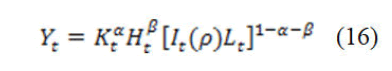
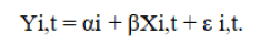
This research shows how Solow's model can include the quality of institutions as a determinant of multifactor productivity. We will consider an economy that produces a single good. The output is a neoclassical production function with diminishing returns to scale of physical capital. Inada's conditions ensure that the marginal products of capital and labor approach infinite as their values approach zero, and zero approach their values go to infinity. The functional form of the Cobb- Douglas production function:
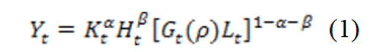
where Yt is real income, Kt is the level of physical capital, Ht is the level of human capital, Lt is the amount of labor employed, Gt is the level of government expenditure, and ρ is the level of the quality of institutions in the country.
Where G (ρ)<. That is 0<α<1, 0< β<1 and 0<β+α<1;
These conditions ensure that the production function exhibits constant returns to scale and diminishing returns to scale at each point. Time is indexed by the continuous variable (t). With the deletion of the term institutional quality, the model yields standard neoclassical results. In other words, the growth rate of per capita output is accelerated by the increase in investment in physical capital and the decrease in population growth, the rate of depreciation of capital, and the initial level of output per capita.
The balance equations are:
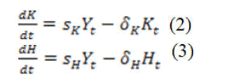
Where, SK, SH, δk, δH are parameters that represent, respectively, the share of income that is attributed to physical and human capital and the rate of depreciation in human and physical capital. In addition, the exogenous population determined and defined:
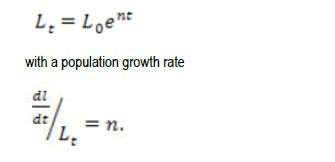
The assumed existence of full employment implies that the growth rate of the labor force is also given by n. At equilibrium w have:

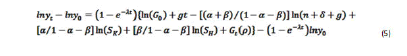
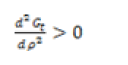
As equation (4) shows that per capita output is in a steady state, an increasing function of the initial level of government expenditure and its growth rate, physical capital, human capital and government expenditure. An expression of per capita output growth can also be expressed by differentiating with respect to time around the steady state.
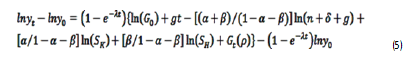
Improving the quality of institutions improves the impact of public spending, per capita output growth. However, with the omission of the quality of institutions variable, equation (5) gives the results of the neoclassical model. In other words, the growth rates of output per capita are accelerated with the increase in investment in physical and human capital and the decrease in population growth, the rate of depreciation of capital, and the initial level of output per capita.
In an effort to model the effect of poor quality institutions on productivity, a structural form of multifactor productivity will be assumed. Schleifer and Mandapaka show that the effect of quality of institutions on the economy is nonlinear and bounded by corruption free production and a level of subsistence production. Since public officials are prone in an economy to corruption (example of quality of institutions) a certain level of output will be produced lower than output without corruption.
To better specify the public expenditure function, we have:
Where 0≤ ρ≤1 et
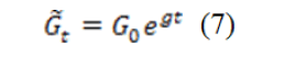
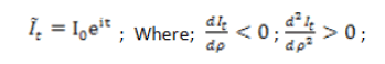
The parameter is the index of the quality of institutions (corruption, rule of law, etc.) determines the magnitude of the effect of this quality on public spending. Public expenditure is exogenous and grows at rate g. We suppose that
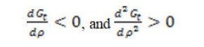
Equation (6) shows that if there is no poor quality of institutions ρ=0 so Ä t=t it's the same for γ=0. The poor quality of institutions does not affect all production functions in the same way. Similarly, a higher value of decreases the effect of the quality of institutions.
When γ tends to zero, the quality function of institutions approaches unity and output is maximal. Equations (1-3) can be expressed in the following intensive form:
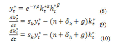
where
= output by head and by public expenditure.
kt*= kt/Gt, is the physical capital per capita by public expenditure.
At steady state, equations (9) and (10) equal zero. Thus, setting them to zero, equations (8),
(9) and (10) form a system of three equations with three unknowns. The equilibrium states of physical and human capital are as follows:
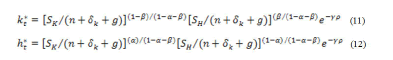
By substituting (11) and (12) in (8), we have the steady state equation.
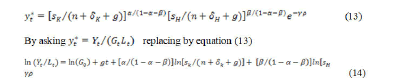
For simplicity, we assume that human and physical capital depreciate at the same rate.
So we have:
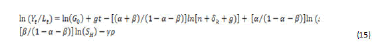
Equation (15) shows that output per capita in the steady state is increasing in the initial level of multifactor productivity, the trend term (gt) and its growth, and rate of investment in physical capital. The more the initial levels of multifactor productivity per capita increase output per capita at the steady state, the more the growth rate of the factors increases, leading subsequently to an increase in output per capita.
Investment shares are found in equations (11) and (12). Higher investment shares increase the levels of physical and human capital per capita, which subsequently increases output per capita from equation (8).
Output per capita, however, is declining in capital amortization per capita (n+δ+g) and quality of institutions. The effect of poor quality institutions depends on the value. A positive value of means poor quality of institutions came out while debilitating causes a negative value means poor quality of institutions came out strengthened. A zero value reduces the output level to the steady state.
The model described above is designed to capture the effect of institution quality on economic growth by integrating institutional quality with multifactor productivity in a Cobb-Douglas production function. These effects reflect the behavior of leaders in government in the allocation of resources. But, agents not only have control over government expenditure but also interfere in the allocation of resources (funds) from other sources such as the World Bank, IMF, United Nations, FAO and UNDP. Foreign governments and other NGO in the form of overseas aid or in the private sector as investments.
Therefore, our model can be modified to examine how the level of the quality of institutions slows economic growth by reducing the level of public spending, aid and investments. Therefore, equation (1) can be reproduced in another form:
Recall equation (6), and replace G (public expenditure) by F (foreign aid), then by I (investment) we have: et
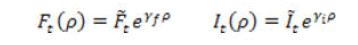
Where λf determine the magnitude of the effect of institutional quality on aid, and λi determines the magnitude of the effect of the quality of institutions on conventional investment Ä©t is exogenous and grows at rate i.
The following equation will be estimated using investment data, respectively:
Extensions of the model: The basic model of the level of real GDP without the "quality of institutions" will be used to estimate the elasticities of production (physical and human capital) using nonlinear least squares as the estimation procedures in the equation next.

Differences in study time period, sample size, and sample selection may lead to different results. Can a change in the level of the quality of institutions lead to a change in the equilibrium level of output per capita? We will add the institution quality variable to the base model, and estimate the following equation.
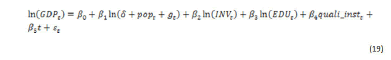
The results of the above equations show that a change in the quality of institutions leads to a change in the equilibrium level of output per capita. A change in the level of the quality of institutions leads to a variation in output through the reduction in the efficiency of public expenditure.
Similarly, the equations (20), (21) below will be used to answer the question: Does a change in the quality of institutions lead to changes in production by reducing the efficiency of investments and the foreign aid?
By comparing the results of the basic model (without institution) with equation (26), we have proof that the poor quality of institutions has impacts on multifactor productivity. Some studies add the variable qualinstit 2 (quality of institutions squared) in the model to verify non-linearity.
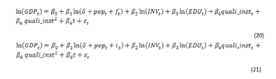
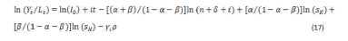
A change in the quality of institutions leads to a change in the growth rate of output per capit. The following equations (22) and (23) will be estimated, where the dependent variable will be the difference in log GDP per capita.
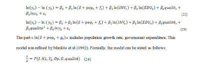
where is the per capita income; I=investment; HL=human capital; Y0=initial level of income, Op=openness to trade; G=public finance variables. And quality=quality of institutions. Using the logarithm, the model can be linearized for the estimation, as follows on panel data:

• y0 is the initial GDP (per capita) or the initial income (per capita).
• k=capital investment or FDI, GFCF.
• hl=gross secondary school enrollment rate.
• op=opening or terms of trade.
• G=public expenditure, TCR, loans granted to the private sector.
• Quality: Qualities of institutions (economic, political or social).
With particular interest, it is evident that institutions matter a lot to foreign investors, and they give the quality of institutions greater importance when considering where to invest. Thus, it is quite logical to assume that foreign investors will create demand for better institutions, and that countries that compete to attract more FDI, and/or recycle the existing stock of FDI, will be required to provide such institutions. The next section will empirically develop this hypothesis.
Empirical test
Based on certain indicators of the quality of institutions, such as democracy, political instability, the proper functioning of legal rules, the quality of bureaucracies, corruption, etc., some studies have succeeded in showing that an efficient institutional framework helps to attract more FDI and subsequently promotes growth.
On the contrary, a poor quality of institutions results in a risky investment climate, lack of confidence of foreign investors, absence of transparency, high transaction costs. However, the proper functioning of these mechanisms is only possible when favorable conditions exist. The empirical strategy takes into consideration the technique of data collection and processing within a very specific methodological framework.
Study sample
The theoretical literature has shown us that there are several determinants of growth; in this framework of analysis we will retain the variables that make it possible to best adjust the dynamics of growth in relation to FDI and the quality of institutions depending on whether one is in a developed or developing country.
Presentation of data: The degree of development of a country is measured from a certain number of statistical indices such as the Human Development Index (HDI), per capita income, etc. The Human Development Index (HDI) is a composite statistical index, created by the United Nations Development Program (UNDP) in 1990, measuring the level of human development of countries around the world. It takes into account the level of study and instruction, life expectancy at birth, and per capita income. This index can be favored by the quality of the institutions.
This analysis relates to a Panel of countries spread over the 4 continents over a period of 22 years (1996-2017);
The UNDP has established three groups of countries according to the HDI (on its website):
• Countries with low human development (HDI<0.5)
• Countries with average human development (HDI between 0.5 and 0.8)
• Developed countries (HDI>0.8).
These first two groups are called developing countries. The choice of the number of countries is due to the availability of data. To have a large panel, we have chosen the period 1996-2012 because the measures on the quality of institutions are almost not available on those prior to 1996 for a larger number of countries.
In our sample we have 110 countries including 40 developed countries (DP) and 70 developing countries (PVD),
The data used in this work are data from the World Bank version 2013, the choice of the number of years is due to the availability of data. We took inspiration from the empirical model to estimate endogenous growth of Barro which was used by Arellano and Bond then Beck, Levine and Loayza in particular. The variables are:
The endogenous variable: GDP/capita: Real GDP per capita is measured in constant US dollars (base 2005), is an acronym for domestic product per capita. In concrete terms, it is a system for measuring the economic activity of a country based on the average income of its citizens.
Exogenous variables
• GDPI0: The initial level of GDP per capita (1996).
• FDI: Also called international direct investment by the OECD, FDI is the international movement of capital made in order to create, develop or maintain a subsidiary abroad and to exercise control over the management of a foreign company. It is the ratio of net flows of foreign direct investment to GDP.
• INV: The ratio of gross fixed capital formation to GDP.
• OUV: This is an indicator for measuring a country's foreign trade. They indicate the country's dependence on the outside world.
The calculation formula is as follows: [(Exports+Imports)/2]/GDP) × 100
• M2: The money supply M2 corresponds to M1 and bank deposits, money market funds and bank reserves
• Credit to the private sector: Sector of the economy that includes households and businesses. The state is not part of the private sector.
• Cr de la pop: "demographic growth" is the evolution of the size of a population for a given territory, the "demographic growth rate" describes the rhythm of this evolution (increase or decrease).
• INF: Inflation is the loss of purchasing power of money which results in a general and lasting increase in prices.
• It must be distinguished from the increase in the cost of living. The loss of value of currency units is a phenomenon that affects the national economy as a whole, without discrimination between categories of agents.
• To assess the inflation rate, the Consumer Price Index (CPI) is used. This measurement is not complete, the inflationary phenomenon covering a wider field than that of household consumption.
• Dep pub: Public expenditure is all expenditure incurred by public administrations. Their financing is ensured by public revenues (taxes, duties and social security contributions) and by the public deficit. Public expenditure, approximated by the share of government consumption in GDP.
• Tx de scol: Human capital is the set of skills, talents, qualifications, experiences accumulated by an individual and which partly determine his ability to work or produce for himself or for others. Is measured in our study by the average number of years of study in the total population.
Institutional variables
The IPC, the reason for use is stated in the previous sections. We measure corruption using the corruption perceptions index established by transparency international. The CPI is on a scale of 0-10: the lower the score, the higher the corruption. This variable may be endogenous. Thus, a higher tax rate gives the opportunity to negotiate a bigger bribe with the taxpayer. An increase in tax pressure thus increases the number of corrupt officials by affecting the moral behavior of officials who were honest. Conversely, a low level of resources resulting from strong corruption limits the action of the State. It then becomes difficult for the State to build solid institutions and create incentive mechanisms favorable to the development of economic activities. Also, a vicious circle emerges where corruption has a negative effect on the economic performance of agents and tax policies, which continues to fuel corruption.
• GOV: Good governance
• Sta pol: The Political Stability (PS) index is an institutional and political factor: Better institutions probably affect economic growth positively.
In contemporary political science, sociology and law there is a large number of views on the nature of political stability, which can be classified as follows:
• Stability understood as the absence of the real threat of illegitimate violence or the presence of state possibilities to eliminate them.
• Stability is a functioning of a government over a long period of time, its know-how presupposing, consequently, successful adaptation to varying realities. One cannot agree with this, since the passage from stability to instability can hardly be explained only by the fall of any government.
• The presence of a constitutional order can be understood as the definitive factor of stability in democratic countries.
• Stability as the consequence of legitimate public power.
• Stability as the absence of structural changes in the political system or as the possibility of directing them.
• Stability as behavior or a social attribute. In this case it can be assimilated to the social situation where the members of society are limited by social norms understanding that each deviation from the norm can lead to instability.
Rule of law: The rule of law can be defined as an institutional system in which public power is subject to the law. It defines sas a state in which legal norms are hierarchized in such a way that its power is limited. In this sense, each rule derives its validity from its conformity to the superior rules. Such a system presupposes, moreover, the equality of subjects of law before legal standards and the existence of independent courts.
Quality of regulation: Measuring the quality and efficiency of the regulatory framework is a flagship publication of the World Bank group and the 13th series of annual reports measuring favorable and unfavorable regulations for business activity. Doing Business presents quantitative indicators on business regulation as well as on the protection of property rights.
Cont of corruption: The notion of corruption is subjective. Be that as it may, it always transgresses the boundary between law and morality. Indeed, one can distinguish active corruption from passive corruption; active bribery consists of offering money or a service to a person who holds power in exchange for an undue advantage; passive corruption consists in accepting this money.
Measuring the quality and efficiency of the regulatory framework is a flagship publication of the World Bank Group and the 13th series of annual reports measuring regulations that help and hinder business activity. Doing Business presents quantitative indicators on business regulation as well as on the protection of property rights.
Descriptive analysis: The difference between institutional changes in developing and developing countries (Figure 3).

Figure 3. Comparison between the average CPI in developing countries and that in developing countries.
In an interval (0, 10) the average CPI of the developed countries is slightly stable between 6 and 7, likewise in the developing countries, the CPI is stable but between 3 and 4, except that there is a rapid increase between the years 2011 and 2012. The difference is clear, so the average CPI of PVD is almost double the CPI of PVD (Figure 4).

Figure 4. Comparison between political stability in developing countries and that in developing countries.
In an interval of (-2.5 and 2.5) the political stability of the PVD revolves around 0.8 throughout the period 1996-2017, in the same way in the PVD it fluctuates between -0.4 and -0. 6 with a considerable decline in the years 2011 and 2012. The difference is wide between these two types of countries, so the DCs are more than twice politically stable than in the PVD (Figures 5 and 6).

Figure 5. Comparison between governance in developing countries and that in developingcountries.

Figure 6. Comparison between the quality of regulation in PVD and that in PVD.
Similarly to political instability, governance has experienced a wide difference between the PVD and the PVD.
Like political stability and governance, the fluctuation in the quality of regulation in DCs averages almost three times that in DCs.
Econometric analysis
Panel data has several advantages. Among these, we can cite the following: the double temporal and individual dimension of the statistics makes it possible to take into account the dynamics and the heterogeneity that could exist between the countries in our case the countries and their economic growth. The number of observations becomes large enough to increase the power of asymptotic tests.
The possibility of taking into account unobserved individual specificities.
In this logic, our priority task consists in clearly specifying the model to be estimated. Given that we combine data from different countries in our sample, it is highly likely that there will be a sample characterized by heterogeneity between the various countries.
Indeed, we can consider a level of homogeneity in the structures, but each country has its own specificities. There are a large number of factors that can influence the explained variable without being explicitly introduced into the model. We can deal with these factors through the residual structure.
Study of panel data
Panel data econometrics seems to be the best way of research for estimating economic growth factors because the use of two dimensions (individual and time) makes it possible to better understand the different possible factors to explain the process. of growth.
First we use a static panel data study then we will advance a dynamic study.
Study of static panel data: The study of panel data requires first of all to check the specification of the data (homogeneous or interogenous). Generally, the use of aggregated data, it is probably unlikely that the growth function is strictly identical for all countries. Especially when the choice of countries is heterogeneous at the level of development (DP and PVD), such as the case of our study sample.
If the homogeneity hypothesis is rejected, and if there is an identical relationship between the endogenous variable and the explanatory variables for all the countries, the source of heterogeneity in the model may result from the constants αi. However, it is logically impossible for all countries to have the same level of structural productivity, for example. We will then begin to test the hypothesis of a common constant for all countries.
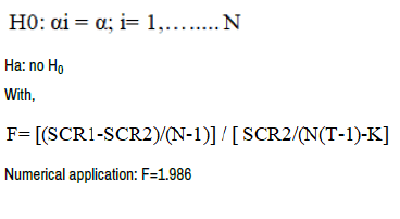
Where SCR 1 is the sum of the squares of the residuals of the model:
(model with individual effects), and SCR2 is the sum of the squares of the residuals of the constrained model:

(Absolutely homogeneous model).
The Fisher statistic associated with the H0 test is equal to (1.986).
This value is to be compared with the Fisher threshold tabulated with (N-1) and N*(T-1)-K degree of freedom. We reject the null hypothesis H0 for this threshold, so there is no equality between the constants αi, this means that our model has individual effects. In this case, these individual effects must be specified (fixed effects or random effects).
According to Haussman, for panels of reduced temporal dimension, there is a strong difference between the two estimators MCG and Whithin. According to him, the strategy of all tests for the specification of individual effects is based on the comparison between these two estimators (MCG and Within), if the two estimators give approximately identical results then the adoption of the random effects model is recommended. In the opposite case where the divergence translates into a correlation then the adoption of fixed effects is necessary.
Hausman specification test
Hausman test is the most popular in the application of tests for the specification of individual effects in a panel. It thus serves to distinguish between fixed and random effects.
Hausman suggests basing the test on the following statistic:
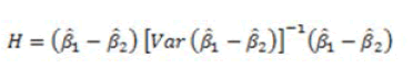
The hypothesis tested examines the correlation of individual effects and explanatory variables.
Ha: no H0
Under H0 the model is specified by random individual effects and therefore the GCM is the best unbiased estimator that should be retained (BLUE estimator). On the other hand, under the alternative hypothesis the model is specified by fixed individual effects and therefore we must retain the within estimator as a best unbiased estimator.
Test results
First, we will test the direct effect of FDI on economic growth without the presence of institutional economic variables.
Subsequently, we will refine the analysis by introducing institutional factors. Does the presence of these variables make the estimates much more robust? Is there a threshold effect of foreign direct investment?
In summary of all the models presented above, it seems obvious that the last one is better in terms of efficiency of the estimates; moreover, this method is used by authors such as Gbewopo Attila Elbir Dorsaf and Goaied Mohameds in their study of the link between corruption and growth.
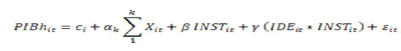
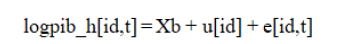
Where i is the country index t time index which represents the year,
Y is the natural logarithm of real GDP per capita, X a vector of predetermined and sexogenic variables (including FDI, the gross rate of schooling, and the Financial Development Index (FDI) such as credits granted to the private sector in logarithmic form). Z gathers the institutional variables and their interactions.
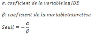
To test the direct effect, in the model we consider:
β=(β1,β2,β3,β4,β5)
X=(logIDEe_PIB, logCred_PIB, logTx_sco_raw,) and Z a vector of exogenous variables
Through our model, institutional factors could have a parabolic effect on economic growth.
Fisher's homogeneity test
F test=0: F (162, 1731)=553.55
Prob>F=0.0000
We reject the null hypothesis H0 (pro<5%), so there is no equality between the constants αi, this means that our model has individual effects. In this case, these individual effects must be specified (fixed effects or random effects) (Table 1).
| Hausman test | ||||
|---|---|---|---|---|
| Coefficients | ||||
| (b) | (B) | (b-B) | Sqrt (diag (V_b-V_B)) | |
| fe | re | Difference | S.E. | |
| logIDEe_PIB | 0.010366 | 0.0132 | -0.00283 | 0.000377 |
| logCred_PIB | 0.24447 | 0.22947 | 0.015 | 0.001903 |
| logtx_sco_~t | 0.257917 | 0.250029 | 0.007888 | 0.006392 |
b=consistent under Ho and Ha; obtained from xtreg B=inconsistent under Ha, efficient under Ho; obtained from xtreg
Test: Ho: Difference in coefficients not systematic
chi2(3)=(b-B)'[(V_b-V_B)^(-1)](b-B)
=95.89
Hausman test Prob>chi2=0.0000
Significance test of random effects
Breusch and pagan lagrangian multiplier test for random effects
Estimated results
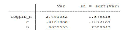
Test: Var (u)=0
chibar2 (01)=5071.19
Prob>chibar2=0.0000
According to Hausman, if the two estimators (MCG and Within), give approximately identical results then the adoption of the random effects model is recommended. The Breuch and Pagan test shows the significance of the random effects (Prob<5%).
The direct effect of FDI on economic growth
Regress logpib_h logpib_h0 logIDEe_PIB logCred_PIB logtx_sco_brut, noconstant (Table 2).
| Source | SS | df | MS | Number of obs=1,897 F (4, 1893)>99999 Prob>F=0.0000 Adj R-Squared=0.9990 R-squared=0.999 Root MSE=0.26942 |
||
|---|---|---|---|---|---|---|
| Model | 132783.9 | 4 | 33195.97 | |||
| Residual | 137.4082 | 1,893 | 0.072588 | |||
| Total | 132921.3 | 1,897 | 70.06921 | |||
| logpib_h | Coef. | Std. Err. | t | P>|t| | 95% Conf. | Interval |
| logpib_h0 | 0.8748 | 0.006431 | 136.02 | 0 | 0.862187 | 0.887413 |
| logIDEe_PIB | 0.037461 | 0.004516 | 8.29 | 0 | 0.028604 | 0.046319 |
| logCred_PIB | 0.092407 | 0.009017 | 10.25 | 0 | 0.074722 | 0.110091 |
| logtx_sco_brut | 0.204556 | 0.011067 | 18.48 | 0 | 0.182851 | 0.22626 |
Regress logpib_h logpib_h0 logIDEe_PIB logCred_PIB logtx_sco_brut, robust
| logpib_h | Coef. | Robust Std. Err. | t | P>|t| | 95% Conf. | Interval |
|---|---|---|---|---|---|---|
| logpib_h0 | 0.875125 | 0.010672 | 82 | 0 | 0.854195 | 0.896056 |
| logIDEe_PIB | 0.03684 | 0.00499 | 7.38 | 0 | 0.027054 | 0.046625 |
| logCred_PIB | 0.090917 | 0.013218 | 6.88 | 0 | 0.064994 | 0.116841 |
| logtx_sco_brut | 0.219013 | 0.018852 | 11.62 | 0 | 0.18204 | 0.255986 |
| _cons | -0.05852 | 0.042454 | -1.38 | 0.168 | -0.14178 | 0.02474 |
Linear regression
Number of obs=1,897
F (4, 1892)=22134.88
Prob>F=0.0000
R-squared=0.9709
Root MSE=.26937
The results show that a 1% increase in FDI/GDP leads to a 0.036% increase in real GDP per capita. The credits allocated to the economy and the gross enrollment rate have a positive influence on growth.
These variables have the merit of fully justifying their presence as explanatory variables in the models. Indeed, the R-squared being close to 1 these variables explains the model. What about the introduction of institutional variables in the estimates of Table 2?
Taking institutional variables into account in the model increases the R2 and makes the model globally significant on average in all the countries of the world, FDI has a direct positive effect on growth by taking into account the effects of institutional variables on growth (continued a 1% increase in FDI growth increases by more than 0.03%). The absence or presence of an institutional variable in the model does not change the volume of the direct impact of FDI on growth.
The OLS estimation method remains weak because it does not take individual specificity into account. To overcome the problem, we will decompose our sample into two groups of developed countries (DP) and developing countries (DC), all by estimating a random effects model. In the following estimates, the GLS method is applied to a random effects model for the case of developed and developing countries. Table 5 presents the estimation results for the PD case.
The results show the existence of an indirect effect of FDI on growth for the estimation with the political stability variable and the governance variable.
In view of these models, there is a quality threshold of institutions below which the effects of FDI on growth are negative. For the Political stability variable, the threshold from which the effect of FDI on growth becomes positive and significant is around 5.55.
Regarding the governance variable, the threshold is around 6.33.
Beyond this threshold, the effects of FDI on growth are positive; ie the more the quality of the institutions is improved, the more the effects are positive on the national economy.
Table 6 presents the estimation results for the PVD case. The results show the existence of an indirect effect of FDI on growth if we add the interactive variables that link FDI with the quality of institutions. The institutional variables that influence the relationship between FDI growth are; political stability, governance, quality of regulations, rule of law and control of corruption (Table 6).
In view of these models, there is a quality threshold of institutions below which the effects of FDI on growth are negative. The calculation of the thresholds allowed us to determine the countries which have not reached the optimal threshold from which they can benefit from FDI, these countries are low income belonging to Africa, Latin America and Asia (Table 8). We notice that the threshold phenomenon is more relevant for the case of PVD.
| Modele-1 | Modele-2 | Modele-3 | Modele-4 | Modele-5 | Modele-6 | Modele-7 | |
|---|---|---|---|---|---|---|---|
| logpib_h | logpib_h | logpib_h | logpib_h | logpib_h | logpib_h | logpib_h | |
| logpib_h0 | 0.875*** | 0.805*** | 0.832*** | 0.861*** | 0.875*** | 0.840*** | 0.875*** |
| -82 | -41.76 | -54.01 | -72.31 | -82.01 | -53.14 | -78.08 | |
| logIDEe_PIB | 0.0368*** | 0.0312*** | 0.0336 | 0.0314*** | 0.0126 | 0.0340*** | 0.0363 |
| -7.38 | -4.39 | -1.49 | -5.95 | -1.45 | -6.35 | -1.22 | |
| logtx_sco_PIB | 0.219*** | 0.353*** | 0.340*** | 0.218*** | 0.220*** | 0.220*** | 0.219*** |
| -11.62 | -9.63 | -9.42 | -11.78 | -11.67 | -11.83 | -11.22 | |
| logCred_PIB | 0.0909*** | 0.112*** | 0.130*** | 0.0835*** | 0.0878*** | 0.0577*** | 0.0909*** |
| -6.88 | -8.38 | -8.67 | -6.56 | -6.52 | -5.66 | -7.4 | |
| logIpc | 0.126*** | ||||||
| -3.63 | |||||||
| logide_logipc | 0.00202 | ||||||
| -0.17 | |||||||
| logsta_pol1 | 0.139*** | ||||||
| -5.67 | |||||||
| logide_logsta_pol1 | 0.0159** | ||||||
| -2.89 | |||||||
| loggov1 | 0.316*** | ||||||
| -4.98 | |||||||
| logide_loggov1 | 0.00036 | ||||||
| -0.02 | |||||||
| _cons | -0.0585 | -0.297*** | -0.353*** | -0.135** | -0.0529 | -0.202*** | -0.0582 |
| (-1.38) | (-3.54) | (-4.18) | (-2.94) | (-1.25) | (-3.38) | (-1.52) | |
| N | 1897 | 1240 | 1240 | 1897 | 1897 | 1897 | 1897 |
| R-sq | 0.971 | 0.971 | 0.97 | 0.972 | 0.971 | 0.972 | 0.971 |
| adj. R-sq | 0.971 | 0.971 | 0.97 | 0.972 | 0.971 | 0.972 | 0.971 |
| prob>F | 0 | 0 | 0 | 0 | 0 | 0 | 0 |
| Modèle-8 | Modèle-9 | Modèle-10 | Modèle-11 | Modèle-12 | Modèle-13 | ||
| logpib_h | logpib_h | logpib_h | logpib_h | logpib_h | logpib_h | ||
| logpib_h0 | 0.850*** | 0.874*** | 0.853*** | 0.876*** | 0.862*** | 0.879*** | |
| -59.28 | -78.47 | -58.42 | -79.38 | -54.87 | -77.94 | ||
| logIDEe_PIB | 0.0327*** | 0.0163 | 0.0349*** | 0.0508 | 0.0356*** | 0.0895** | |
| -5.94 | -0.5 | -6.68 | -1.83 | -6.69 | -2.69 | ||
| logtx_sco_~t | 0.220*** | 0.220*** | 0.224*** | 0.218*** | 0.227*** | 0.214*** | |
| -11.83 | -11.47 | -11.59 | -11.2 | -10.8 | -10.88 | ||
| logCred_PIB | 0.0713*** | 0.0891*** | 0.0658*** | 0.0925*** | 0.0793*** | 0.0963*** | |
| -6.29 | -7.07 | -6.01 | -7.39 | -7.57 | -7.96 | ||
| logqual_regul1 | 0.231*** | ||||||
| -4.51 | |||||||
| logide_logqual_regul1 | 0.0127 | ||||||
| -0.7 | |||||||
| logetat_droit1 | 0.207*** | ||||||
| -3.9 | |||||||
| logide_logetat_droit1 | -0.0086 | ||||||
| (-0.57) | |||||||
| logcont_corrup1 | 0.107* | ||||||
| -1.96 | |||||||
| logide_logcont_corrup1 | -0.0317 | ||||||
| (-1.77) | |||||||
| _cons | -0.183** | -0.0476 | -0.159** | -0.065 | -0.124* | -0.0818* | |
| (-3.09) | (-1.29) | (-2.84) | (-1.66) | (-2.02) | (-2.11) | ||
| N | 1897 | 1897 | 1897 | 1897 | 1897 | 1897 | |
| R-sq | 0.972 | 0.971 | 0.971 | 0.971 | 0.971 | 0.971 | |
| adj. R-sq | 0.972 | 0.971 | 0.971 | 0.971 | 0.971 | 0.971 | |
| prob>F | 0 | 0 | 0 | 0 | 0 | 0 |
|
|
Modele 1 |
Modele 2 |
Modele 3 |
Modele 4 |
Modele 5 |
Modele 6 |
Modele 7 |
||||||
|---|---|---|---|---|---|---|---|---|---|---|---|---|---|
|
|
logpib_h |
logpib_h |
logpib_h |
logpib_h |
logpib_h |
logpib_h |
logpib_h |
||||||
|
logpib_h0 |
0.789*** |
0.771*** |
0.797*** |
0.772*** |
0.782*** |
0.719*** |
0.775*** |
||||||
|
|
-43.21 |
-32.65 |
-36.37 |
-41.72 |
-43.8 |
-34.3 |
-41.16 |
||||||
|
logIDEe_PIB |
0.0139** |
0.0123* |
-0.0087 |
0.0130** |
-0.0989 |
0.0135** |
-0.12 |
||||||
|
|
-2.95 |
-2.42 |
(-0.29) |
-2.77 |
(-1.86)* |
-3 |
(-1.96)* |
||||||
|
logCred_PIB |
0.265*** |
0.249*** |
0.256*** |
0.268*** |
0.261*** |
0.253*** |
0.260*** |
||||||
|
|
-23.69 |
-19.24 |
-19.89 |
-24.17 |
-23.36 |
-23.26 |
-23.22 |
||||||
|
logtx_sco_~t |
0.245*** |
0.145* |
0.161** |
0.238*** |
0.253*** |
0.200*** |
0.247*** |
||||||
|
|
-4.7 |
-2.56 |
-2.83 |
-4.61 |
-4.91 |
-3.92 |
-4.78 |
||||||
|
logIpc |
|
0.146** |
|
|
|
|
|
||||||
|
|
|
-3.29 |
|
|
|
|
|
||||||
|
logide_logipc |
|
|
0.0113 |
|
|
|
|
||||||
|
|
|
|
-0.74 |
|
|
|
|
||||||
|
logsta_pol1 |
|
|
|
0.211*** |
|
|
|
||||||
|
|
|
|
|
-3.86 |
|
|
|
||||||
|
logide_logsta_pol1 |
|
|
|
|
0.0577* |
|
|
||||||
|
|
|
|
|
|
-2.14 |
|
|
||||||
|
loggov1 |
|
|
|
|
|
0.586*** |
|
||||||
|
|
|
|
|
|
|
-7.24 |
|
||||||
|
logide_loggov1 |
|
|
|
|
|
|
0.0650* |
||||||
|
|
|
|
|
|
|
|
-2.19 |
||||||
|
_cons |
-0.045 |
0.393 |
0.304 |
-0.264 |
0.0107 |
-0.293 |
0.104 |
||||||
|
|
(-0.21) |
-1.61 |
-1.22 |
(-1.18) |
-0.05 |
(-1.32) |
-0.46 |
||||||
|
N |
582 |
491 |
491 |
582 |
582 |
582 |
582 |
||||||
|
|
Modele 8 |
Modele 9 |
Modele 10 |
Modele 11 |
Modele 12 |
Modele 13 |
|||||||
|
|
logpib_h |
logpib_h |
logpib_h |
logpib_h |
logpib_h |
logpib_h |
|||||||
|
logpib_h0 |
0.767*** |
0.784*** |
0.742*** |
0.781*** |
0.788*** |
0.793*** |
|||||||
|
|
-41.18 |
-43.81 |
-35.78 |
-42.79 |
-38.79 |
-42.59 |
|||||||
|
logIDEe_PIB |
0.0128** |
-0.0414 |
0.0144** |
-0.0698 |
0.0139** |
0.0504 |
|||||||
|
|
-2.73 |
(-0.66) |
-3.11 |
(-1.08) |
-2.93 |
-1.09 |
|||||||
|
logCred_PIB |
0.253*** |
0.258*** |
0.246*** |
0.257*** |
0.265*** |
0.265*** |
|||||||
|
|
-22.33 |
-22.78 |
-20.93 |
-22.48 |
-23.31 |
-23.45 |
|||||||
|
logtx_sco_~t |
0.253*** |
0.266*** |
0.224*** |
0.258*** |
0.245*** |
0.250*** |
|||||||
|
|
-4.92 |
-5.18 |
-4.35 |
-5.02 |
-4.67 |
-4.8 |
|||||||
|
logqual_regul1 |
0.267*** |
|
|
|
|
|
|||||||
|
|
-3.92 |
|
|
|
|
|
|||||||
|
logide_logqual_regul1 |
|
0.0273 |
|
|
|
|
|||||||
|
|
|
-0.89 |
|
|
|
|
|||||||
|
logetat_droit1 |
|
|
0.436*** |
|
|
|
|||||||
|
|
|
|
-4.93 |
|
|
|
|||||||
|
logide_logetat_droit1 |
|
|
|
0.041 |
|
|
|||||||
|
|
|
|
|
-1.31 |
|
|
|||||||
|
logcont_corrup1 |
|
|
|
|
0.00683 |
|
|||||||
|
|
|
|
|
|
-0.1 |
|
|||||||
|
logide_logcont_corrup1 |
|
|
|
|
|
-0.0177 |
|||||||
|
|
|
|
|
|
|
(-0.79) |
|||||||
|
_cons |
-0.349 |
-0.0593 |
-0.289 |
0.00592 |
-0.0463 |
-0.103 |
|||||||
|
|
(-1.54) |
(-0.28) |
(-1.28) |
-0.03 |
(-0.21) |
(-0.46) |
|||||||
|
N |
582 |
582 |
582 |
582 |
582 |
582 |
|||||||
| cc | Modele 1 | Modele 2 | Modele 3 | Modele 4 | Modele 5 | Modele 6 | Modele 7 | ||||||
|---|---|---|---|---|---|---|---|---|---|---|---|---|---|
| logpib_h | logpib_h | logpib_h | logpib_h | logpib_h | logpib_h | logpib_h | |||||||
| logpib_h0 | 0.791*** | 0.760*** | 0.771*** | 0.790*** | 0.790*** | 0.771*** | 0.776*** | ||||||
| -34.61 | -23.66 | -24.28 | -34.27 | -34.53 | -32.29 | -33.89 | |||||||
| logIDEe_PIB | 0.0133** | 0.0175** | -0.0272 | 0.0132** | -0.0212* | 0.0122** | -0.135*** | ||||||
| -3.03 | -2.83 | (-1.59) | -3 | (-2.06) | -2.77 | (-6.13) | |||||||
| logCred_PIB | 0.207*** | 0.192*** | 0.202*** | 0.206*** | 0.201*** | 0.200*** | 0.198*** | ||||||
| -18.39 | -13.78 | -14.77 | -18.19 | -17.86 | -17.48 | -17.76 | |||||||
| logtx_sco_~t | 0.270*** | 0.407*** | 0.405*** | 0.270*** | 0.271*** | 0.276*** | 0.285*** | ||||||
| -12.23 | -12.67 | -12.51 | -12.23 | -12.37 | -12.5 | -13.1 | |||||||
| logIpc | 0.127*** | ||||||||||||
| -3.9 | |||||||||||||
| logide_logipc | 0.0394** | ||||||||||||
| -2.94 | |||||||||||||
| logsta_pol1 | 0.00823 | ||||||||||||
| -0.32 | |||||||||||||
| logide_logsta_pol1 | 0.0248*** | ||||||||||||
| -3.69 | |||||||||||||
| loggov1 | 0.172** | ||||||||||||
| -3.03 | |||||||||||||
| logide_loggov1 | 0.0982*** | ||||||||||||
| -6.86 | |||||||||||||
| _cons | -0.00456 | -0.446 | -0.41 | -0.00899 | 0.00573 | -0.124 | 0.0623 | ||||||
| (-0.03) | (-1.90) | (-1.75) | (-0.06) | -0.04 | (-0.74) | -0.38 | |||||||
| N | 1315 | 749 | 749 | 1315 | 1315 | 1315 | 1315 | ||||||
| Modele 8 | Modele 9 | Modele 10 | Modele 11 | Modele 12 | Modele 13 | ||||||||
| logpib_h | logpib_h | logpib_h | logpib_h | logpib_h | logpib_h | ||||||||
| logpib_h0 | 0.753*** | 0.778*** | 0.783*** | 0.780*** | 0.794*** | 0.783*** | |||||||
| -31.87 | -33.93 | -32.97 | -34.1 | -33.73 | -34.6 | ||||||||
| logIDEe_PIB | 0.00909* | -0.129*** | 0.0126** | -0.104*** | 0.0134** | -0.104*** | |||||||
| -2.1 | (-6.55) | -2.86 | (-5.00) | -3.05 | (-4.11) | ||||||||
| logCred_PIB | 0.192*** | 0.197*** | 0.204*** | 0.199*** | 0.208*** | 0.204*** | |||||||
| -17 | -17.75 | -17.72 | -17.74 | -18.2 | -18.3 | ||||||||
| logtx_sco_~t | 0.291*** | 0.279*** | 0.273*** | 0.280*** | 0.268*** | 0.271*** | |||||||
| -13.3 | -12.88 | -12.3 | -12.81 | -12.07 | -12.41 | ||||||||
| logqual_regul1 | 0.303*** | ||||||||||||
| -6.93 | |||||||||||||
| logide_logqual_regul1 | 0.0945*** | ||||||||||||
| -7.4 | |||||||||||||
| logetat_droit1 | 0.068 | ||||||||||||
| -1.29 | |||||||||||||
| logide_logetat_droit1 | 0.0782*** | ||||||||||||
| -5.76 | |||||||||||||
| logcont_corrup1 | -0.0277 | ||||||||||||
| (-0.56) | |||||||||||||
| logide_logcont_corrup1 | 0.0756*** | ||||||||||||
| -4.7 | |||||||||||||
| _cons | -0.235 | 0.0763 | -0.0516 | 0.0535 | 0.0188 | 0.0512 | |||||||
| (-1.41) | -0.47 | (-0.31) | -0.33 | -0.11 | -0.32 | ||||||||
| N | 1315 | 1315 | 1315 | 1315 | 1315 | 1315 | |||||||
Threshold calculation (Estimation BETWIN)
| Coef | SP | GOV | QR | ed | CC |
|---|---|---|---|---|---|
| α | -0,0212 | -0,135 | -0,129 | -0,104 | -0,104 |
| β | 0,0248 | 0,0982 | 0,0945 | 0,0782 | 0,0756 |
| Seuil (en log) =1-α/β | 0,854838 | 13,74,745 | 13,65,07,937 | 13,29,92,327 | 13,75,66,138 |
| Exp (seuil) | 23,50,99,516 | 39,54,06,996 | 39,16,03,384 | 37,80,75,329 | 39,57,69,338 |
Threshold calculation (Estimation BETWIN).
| Coef | Stab.pol | gov |
|---|---|---|
| α | -0.0989 | -0.120 |
| β | 0.0577 | 0.0650 |
| Seuil (en log)=1-α/β | 1,71403813 | 1,84615385 |
| Exp (seuil) | 5,55133327 | 6,33540566 |
For DP the threshold exists for the institutional variables SP and GOV, no threshold for the other variables positive and significant relationship between growth and FDI. On average, SP for PD is around 6.92>5.5 (threshold), and average gov=7.7>6.33 (threshold). It can be seen that for developed countries the relationship between FDI and economic growth is linear and positive, the threshold phenomenon is verified for the two institutional indicators political stability and good governance (Table 9).
| Sp | Sp | Gov | Gov | Qr | Qr | Ed | Ed | Cc | Cc |
|---|---|---|---|---|---|---|---|---|---|
| AFGHANIST AN | 1,12 | CONGO, DEM, REP, | 2,373 | TURKMENIS TAN | 1,947 | AFGHANIST AN | 2,249 | AFGHANIST AN | 2,554 |
| CONGO, DEM, REP, | 1,23 | AFGHANIS TAN | 2455 431 | AFGHANIST AN | 2286 446 | CONGO, DEM, REP, | 2321 995 | CONGO, DEM, REP, | 2,787 |
| SUDAN | 1,43 | IRAQ | 2,595 | ZIMBABWE | 2,399 | IRAQ | 2,599 | EQUATORIA L GUINE | 2,867 |
| IRAQ | 1,61 | COMORO S | 2,713 | UZBEKISTA N | 2410 715 | HAITI | 2657 275 | IRAQ | 2,982 |
| BURUNDI | 1,99 | LIBERIA | 2,745 | DEM, REP, CONGO, | 2451 659 | LIBERIA | 2706 071 | HAITI | 3,072 |
| PAKISTAN | 2,13 | EQUATORI AL GUINE | 2,815 | IRAQ | 2584 301 | ZIMBABWE | 2,829 | ANGOLA | 3,146 |
| COLOMBIA | 2,29 | HAITI | 2,874 | ERITREA | 2,656 | ANGOLA | 2,845 | SUDAN | 3,356 |
| TURKMEN ISTAN | 2,901 | LIBERIA | 2,662 | GUINEA-BISSAU | 2,853 | TURKMENIS TAN | 3,362 | ||
| CENTRAL AFRICAN | 2902 094 | IRAN, ISLAMIC RE | 2735 871 | SUDAN | 2921 768 | CHAD | 3,432 | ||
| BURUNDI | 3071 655 | LIBYA | 2751 975 | CENTRAL AFRICAN | 2922 7 | PARAGUAY | 3467 824 | ||
| TOGO | 3133 089 | EQUATORIA L GUINE | 2855 632 | TURKMENIS TAN | 2983 56 | TAJIKISTAN | 3483 952 | ||
| SIERRA LEONE | 3136 978 | CUBA | 2867 558 | GUINEA | 3043 472 | NIGERIA | 3488 338 | ||
| CONGO, REP, | 3247 464 | BELARUS | 2936 925 | BURUNDI | 3091 875 | BURUNDI | 3519 49 | ||
| SUDAN | 3272 838 | COMOROS | 3036 536 | EQUATORIA L GUINE | 3127 966 | ZIMBABWE | 3542 506 | ||
| GUINEA-BISSAU | 3328 04 | SOLOMON ISLANDS | 3073 29 | CONGO, REP, | 3148 816 | AZERBAIJAN | 3543 528 | ||
| ANGOLA | 3347 731 | SUDAN | 3090 006 | CHAD | 3153 821 | CENTRAL AFRICAN | 3562 425 | ||
| TAJIKISTA N | 3419 524 | ANGOLA | 3106 732 | TAJIKISTAN | 3174 689 | GUINEA-BISSAU | 3583 566 | ||
| ERITREA | 3443 566 | BURUNDI | 3193 718 | VENEZUELA, RB | 3236 241 | CAMBODIA | 3584 929 | ||
| SOLOMO N ISLANDS | 3489 586 | CONGO, REP, | 3314 135 | CTE D'IVOIRE | 3251 521 | UZBEKISTAN | 3595 328 | ||
| CHAD | 3,492 | LAO PDR | 3,323 | UZBEKISTA N | 3,254 | LIBERIA | 3,608 | ||
| LIBYA | 3,58 | SYRIAN ARAB REPU | 3,382 | YEMEN, REP, | 3,258 | CAMEROON | 3,619 | ||
| WEST BANK AND GA | 3,62 | TAJIKISTAN | 3,39 | NIGERIA | 3,263 | CONGO, REP, | 3,619 | ||
| GUINEA | 3,63 | SIERRA LEONE | 3,48 | CAMEROON | 3396 386 | BANGLADES H | 3,66 | ||
| UZBEKIST AN | 3,65 | GUINEA-BISSAU | 3,49 | SIERRA LEONE | 3,40 | PAPUA NEW GUINEA | 3,70 | ||
| NIGERIA | 3,66 | CENTRAL AFRICAN | 3,52 | COMOROS | 3,51 | LAO PDR | 3,71 | ||
| ZIMBABW E | 3,71 | ETHIOPIA | 3,56 | CAMBODIA | 3513 321 | KAZAKHSTA N | 3,72 | ||
| PARAGUA Y | 3,76 | CHAD | 3,67 | GUATEMAL A | 3,56 | VENEZUELA, RB | 3,74 | ||
| VENEZUEL A, RB | 3,78 | HAITI | 3,71 | BELARUS | 3,61 | KENYA | 3,76 | ||
| DJIBOUTI | 3,81 | VENEZUELA, RB | 3,80 | PARAGUAY | 3,68 | LIBYA | 3,77 | ||
| BELARUS | 3846 382 | BANGLADES H | 3,81 | KYRGYZ REPUBLIC | 3686 365 | UKRAINE | 3,78 | ||
| CTE D'IVOIRE | 3,86 | GUINEA | 3,84 | LAO PDR | 3,74 | PAKISTAN | 3,80 | ||
| CAMBODI A | 3,86 | NIGERIA | 3,90 | KENYA | 3,76 | RUSSIAN FEDERATI | 3,81 | ||
| SYRIAN ARAB REPU | 3,91 | KYRGYZ REPUBLIC | 3,83 | ||||||
| YEMEN, REP, | 3,92 | SIERRA LEONE | 3,90 | ||||||
| LAO PDR | 3,92 | COMOROS | 3,90 | ||||||
| NIGER | 3,94 | GUINEA | 3,91 | ||||||
| YEMEN, REP, | 3,92 | ||||||||
| NIGER | 3,93 | ||||||||
| ECUADOR | 3,93 | ||||||||
| HONDURAS | 3,94 | ||||||||
| SYRIAN ARAB REPU | 3,95 |
Regarding the case of developing countries, the results show the existence of an indirect effect of FDI on growth if we add the interactive variables that link FDI with the quality of institutions. The institutional variables that influence the relationship between FDI growth are; political stability, governance, quality of regulations, rule of law and control of corruption. This allows us to conclude that the threshold phenomenon is more relevant for developing countries. These countries must reach a certain threshold of institutional development to be able to benefit from FDI (the developing countries below the threshold are presented as follows) (Table 10).
| Pays | Sta_pol1 | Pays | Gov1 |
|---|---|---|---|
| ISRAEL | 31,78,854 | MADAGASCAR | 43,11,999 |
| MADAGASCAR | 52,11,355 | ARGENTINA | 54,64,701 |
| ARGENTINA | 52,31,727 | SEYCHELLES | 57,86,427 |
| SPAIN | 55,35,842 | CROATIA | 62,18,902 |
As part of this research project, we are expected to a very controversial question. This is the nature of the effect of a country's FDI on its economic growth. To answer this question, we brought our research on two essential parts: A theoretical part and an elementary part. At the level of the theoretical part, we started with a traditional study of the impact of FDI on growth in order to understand the economic changes that have characterized the process of growth in recent years, on the real and institutional level. These institutional changes were accompanied by a new wave of studies carried out by theoretical economists like Stiglitz and many others like Spence and Akerlof. The contribution of this work has recently sparked renewed interest in the role of economic and political institutions not only in the theory of economic growth, but also in other fields such as macroeconomics and development economics. In order to solve the question posed at the start, we proceeded in this work to the following methodology: analyze the problem, determine a theoretical relation, define the subject concepts and finally validate all that is possible to do empirically. The association between FDI and economic growth has been the subject of several theoretical works that have focused on the level of human capital, technology transfer, etc. Indeed, Eicher. T and Penasola. C.G argues that institutions can promote economic growth as they improve the level of stability, predictability and certainty for foreign investors who encourage them to invest more, which positively affects the economic performance of the country. in question. A descriptive study of FDI and economic growth does not allow us to decelerate a possible link between the two. To overcome this fact, we used a dynamic panel data model covering a sample of 110 countries in the world during the period 1996-2017. In this empirical study, we tested the direct and indirect effects of FDI on economic growth. The key findings from this econometric analysis revealed that:
• In DCs we have a directly positive effect of FDI on economic growth, then our research did not lead to a significant conclusion of the indirect effect of FDI on growth. This could be due to the weakness of the instruments used in the model and the sample size.
• In developing countries, the effect of FDI on growth depends on the level of the quality of institutions compared to a threshold level that could be called the level of (tolerance). If foreign direct investment expands to a certain level, the tolerance threshold increases, resulting in an increasingly positive impact of FDI on growth over time.
• However, it is important to point out that, despite the importance of the presumed empirical results about our research, shortcomings could be raised: the problem of causality has not been addressed.
• Other possible mechanisms of the studied relationship were not assumed.
• The lack of data for certain countries does not allow us to take into account certain explanatory variables of growth in the model. Our results, far from being exhaustive, will allow us to better understand the relationship between FDI and economic growth, through a system GMM model. This solves the problem of the instruments, but if we used it, it is because this model makes the variable IDE insignificant.
[Crossref] [Googlescholar] [Indexed]
[Crossref] [Googlescholar] [Indexed]
[Crossref] [Googlescholar] [Indexed]
[Crossref] [Googlescholar] [Indexed]
[Crossref] [Googlescholar] [Indexed]
[Crossref] [Googlescholar] [Indexed]
[Crossref] [Googlescholar] [Indexed]
[Crossref] [Googlescholar] [Indexed]
[Crossref] [Googlescholar] [Indexed]
[Crossref] [Googlescholar] [Indexed]
[Crossref] [Googlescholar] [Indexed]
[Googlescholar] [Indexed]
[Crossref] [Googlescholar] [Indexed]
[Googlescholar] [Indexed]
[Googlescholar] [Indexed]
[Crossref] [Googlescholar] [Indexed]
[Googlescholar] [Indexed]
Business and Economics Journal received 6451 citations as per Google Scholar report