Consistence Condition of Kernel Selection in Regular Linear Kernel Regression and Its Application in COVID-19 High-risk Areas Exploration

Lu xan^* and Ba lin
^*Correspondence: Dr. Lu xan, Department of Mathematic and Statistics, Central China Normal University, Luoyu, Wuhan, 430071, Hubei, China, Email:

Keywords

Linear kernel • COVID-19 source exploration • Kernel selection • Superimposed fields

Introduction

COVID-19 was recognized in December 2019 [1]. Since then, the COVID-19 out-break has posed critical challenges for the public health, research, and medical communities. Currently, it was recognized that human to human transmission played a major role in the subsequent outbreak [2]. Based on this knowledge, in the data collection stage, we try to extract data related to the flow of people as much as possible. At present, the research on the COVID-19 mainly focuses on the treatment of the epidemic [3,4]; the transmission of the epidemic [5,6] and the prevention of the epidemic [7,8]. In F. Ndairou 2020, the concept of super-spreaders, who contribute disproportionately to a much larger number of cases in the ongoing COVID-19 pandemic, was proposed for modeling the COVID-19 transmission. We focus our attention on high-risk areas exploration from “sky” perspective. Which means that, we ignore different regional political factors and medical level factors? All the factors we can know come from aerial monitoring. We imagine ourselves as a space traveler. Before landing on the earth, determining which areas are high-risk areas and which areas are low- risk areas through detection in the sky is actually our task. In order to make a decision, we had to count the number of outbreaks in each region, as well as all the data related to the spread of the outbreak, e.g. population, population density per square kilometer, population transmission, people gathering frequency, distances between regions, etc. Given this information of different areas, we cannot decide the risk level of one area, just by the outbreaks. Because, for several adjacent areas, the surrounding areas are likely to be only the victim and only one area is the source of the outbreak. One the other hand, for areas of high volume of population transmission and people gathering frequency, its low-risk label may only be temporary. Along the continuous outbreak of COVID-19, those areas are much like to become high-risk areas.

The inspiration of Regular Linear Kernel Regression, which is used for high risk area detection of COVID-19 in this paper, comes from a variable selection method, called Lasso [9], which is firstly proposed for solving S-sparse linear regression model in high-dimensional statistics. Actually the proof framework of Kernel Selection Consistence origins from the variable selection consistence of Lasso [10], but a slightly modification for suitable for Kernel Selection. To gain an intuition of the link between Kernel Selection and high-risk areas exploration, let us see inside of Kernel Regression.

Denote Kα(x)=K(α, x) be a measure of the distance between α and x, where the Gaussian RBF(Radial Basis Function) Kernel and Linear Inner Product Kernel are most widely used. In this paper, the kernel selection consistence condition of Regular Linear Kernel Regression was given. For a given group of kernels, Kα (.), α£α ¯, where α¯ stands for an index set, Kernel Regression model has the form,

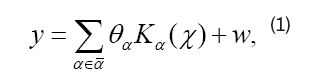
Where, y stands for outbreaks and w stands for observation noise. From the model, y is actually a linear combination of the characteristic Kernels at the point of x. We see a Kernel Kα(x) as a spread function of a high-risk area characterized by α. As stated, Kα(x) is a measure of the distance between α and x. For a long distance area x from high-risk area α, the influence from α, source of transmission, shall be small, which is coincident with the property of Kα(x). Upper to now, we explain the link between the spreading mode of COVID-19 and the Kernel Regression, that’s high-risk areas were seen as emission sources characterized by Kα(.) in the model and the outbreaks in one area is actually the combination of the influences of those emission sources. Still, there are problems that must be check carefully. First, the number of high-risk areas can be unlimited? For a given design matrix X ∈ R^n×d, and a candidate set Card (α)=m, the number of high-risk areas s must be less than or equal to min (n, d, m), otherwise the true high-risk areas will not be check out entirely. Second, for a given estimation of (θ) with a support set of Sˆ, under which conditions the support set is consistent with the true support set S of true θ? This question is crucial, as it means whether we have got the true high-risk areas or COVID-19 sources. As a non-zero θα means that the candidate area of Kα (.) influences other areas. 

Notice that, Interpolation learning has recently attracted growing attention in the machine learning community [11,12]. Linear Kernel Regression model has been around for decades, whose continued popularity stems from its excellent properties, well generalization along with good interpolation, in high- dimensional statistics. Due to the derivability, Kernel Ridge Regression with l2-norm penalization is very popular in the High-dimensional area, including the converge rate [13], generalization risk [14] and variable selection [15]. While the Consistence condition of Kernel Regression with l1-norm penalization is the novelty of this paper, that’s the topic of Kernel selection consistency under l1-norm regularization is first proposed in this paper. We compliment the consistence condition for Kernel Regression with l1-norm penalization, along with the generalization risk. Due to the interpolation of Kernel regression [16], the connection between Kernel selections with high-risk areas detection of COVID-19 is our innovation. Around those questions, we structured our paper as follows. In the introduction, we briefly introduce the background of COVID-19 transmission and give the inspiration of high-risk areas exploration. In the second section, some remarks were introduced and Linear Kernel Regression Model was proposed for the spreading mode of COVID-19 on high-risk areas influence view. As we have no hope for estimating an unique solution of θˆ with the optimal least square method. Regular technique was suggested for estimating an unique solution. In the third section, the conditions of Kernel Selection Consistence were given. Finally the simulation experiment was conduct for supplements of consistence checking. Then the Kernel Selection Method was applied for COVID-19 high-risk areas detection with outbreaks of COVID-19 up to year 2021 along with some other features that influence the transmission of COVID-19.

Materials and Methods

Model construction

Suppose we are given relevant features in observation regions, x_i=(x_i1, x_i2,… x_id)T and corresponding response values yi, for i=1, …, n, which stands for the most concerned variable, e.g. the number of epidemic out breaks. A significant research is to find possible emission sources or high- risk areas from many candidate areas α_j=(α_j1,…, α_jd)T , for j=1,… , m. The true high-risk areas αS is supposed to be contained in those candidate areas α¯=(αT₁ , . . . , αT_m )T indexed by S and S ⊆ (m) stands for the true support of high-risk areas. Here (m) is a simplified notation of (1, … , m).

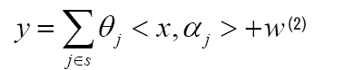
Intuitively, the response variable y at observation point x is the linear superimposed effects of each real high-risk areas, that’s

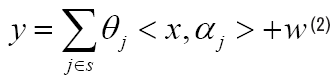
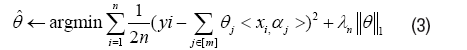
where S (1, . . . , m) stands for the supports of truth emission sources, and w stands for observation noise. <. , .> stands for inner product. Since S is unknown in practice, the estimation problem of S will be more meaningful, except for the estimation of ^j, j ∈ S. Actually if the support S of the truth emission sources was given, we can estimate ˆθ very well. With the true S unknown, there is no hope for obtaining an unique solution of j , when m ≥ min(n, d), from Lemma 1 in Appendix. Without uniqueness, there is no way to talk about the Kernel Selection Consistence. Inspired by Lasso of l1 norm regularization, consider the following optimization,

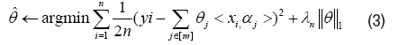
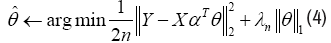
Here, [m]={1, . . . , m} is a simple notation and λn is a given parameter. Denote X=[x₁,…, x_n]^T ∈ R^n×d, α=[α1,…, αm]T ∈ Rm×d, θ=[θ1,… , θm]T Rm and Y=[y1,…, y_n]T ∈ Rⁿ. Therefore a matrix form alternative of equation (3), namely Regular Linear Kernel Regression, is given by,

where S (1, . . . , m) stands for the supports of truth emission sources, and w stands for observation noise. <. , .> stands for inner product. Since S is unknown in practice, the estimation problem of S will be more meaningful, except for the estimation of ^j, j ∈ S. Actually if the support S of the truth emission sources was given, we can estimate ˆθ very well. With the true S unknown, there is no hope for obtaining an unique solution of j , when m ≥ min(n, d), from Lemma 1 in Appendix. Without uniqueness, there is no way to talk about the Kernel Selection Consistence. Inspired by Lasso of l1 norm regularization, consider the following optimization,

Here, [m]={1, . . . , m} is a simple notation and λn is a given parameter. Denote X=[x1,…, x_n]T ∈ R^n×d, α=[α1,…, αm]T ∈ Rm×d, θ=[θ1,… , θm]T Rm and Y=[y1,…, y_n]^T ∈ Rⁿ. Therefore a matrix form alternative of equation (3), namely Regular Linear Kernel Regression, is given by,

For the not differentiable of l1- norm, due to its sharp point at the origin, there’s no hope for a close form solution. Since this is a convex optimization problem, many optimization methods can be used to solve the problem, e.g. Gradient descent or Least Angel Regression.

So the method of estimating θˆ is not the focus of this paper. The explanation of the estimation result of θˆ and the condition of consistence between the estimation and the truth θ is our focus. Here we give the explanation of θˆ. From the model(2), for a zero θ_j=0, which means y is irrelevant with αj, the location of α_j shall not be the emission source. For a non-zero θ_j, which means y is relevant with α_j, the location of αj shall be the emission source. For a positive θ_j, the corresponding location of α_j shall be seen as pollution source in the pathogen exploration case. And a negative θ_j, the corresponding location of αj shall be seen as purification source.

Results

Condition of consistence

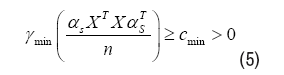
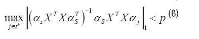
Consider an S-sparse linear kernel regression model and the true support of θ٨ is S. Given an estimation θˆ with support Sˆ. The question is by which condition the estimation Sˆ is consistent with S We begin by assuming X be deterministic design matrices. Let S stands for the supports of truth θ٨ and αS stands for the subset of α=[α1, αm]T with indices of S. First the truth emission source αS cannot be linearly correlated, in order to ensure that the model is identifiable, even if the support set S were known a priori. Second the fake source αSC shall be irrelevant with the truth emission source αS, which makes it possible to exclude irrelevant areas. In general, we cannot expect this orthogonality to hold, but a type of approximate orthogonality. In particular, consider the following conditions:

Lower eigenvalue: The smallest eigenvalue of the sample covariance submatrix indexed by S is bounded below:

Mutual incoherence: There exists some p ∈ [0, 1) such that

With this set-up, the following results follow applied to the lagrange form Linear Kernel Lasso (4) when applied to an instance of the linear kernel model (2) such that the true parameter θ* is supported on a subset S with cardi- nality s. In order to state the result, we introduce the convenient shorthand a type of orthogonal projection matrix.

Theorem 1

Consider an S-sparse linear kernel regression model for which the design matrix satisfies conditions (5) and (6). Then for any choice of regularization parameter such that

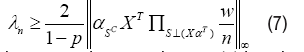
the Lagrangian Kernel Lasso (3) has the following properties:

(a)Uniqueness: There is a unique optimal solution ∈ˆ

(b)No false inclusion: The solution has its support set Sˆ contained within the true support set S.

c) l∞-bounds: The error ˆθ – θ* satisfies

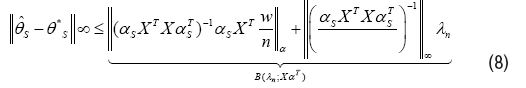
(d)No false exclusion: The solution’s support set Sˆ includes all indicesi ∈ S such that |θi*|>B(λn; X^T), and hence is sample selection consistent if mini∈ S | θi*|>B(λn; XαT),

The prove of this result utilizes a technique called a primal-dual witness method, which constructs a solution and then the solution was shown be optimal and unique, see Appendix. Here let us try to interpret its main claims. First the uniqueness claim in part(a) is not trivial. Although the Lagrange objective is convex, it can never be strictly convex when m>min{d, n}. Based on the uniqueness claim, we can talk unambiguously about the support of the Kernel Lasso estimate θˆ. Part (b) guarantees that the kernel lasso does not falsely include linear kernels that are not in the support of θ*, or equivalently that θˆsC=0. Part (d) is a consequence of the l∞-norm bound from part (c): as long as the minimum value of |θi*|over indices i∈S is not too small, then the Kernel Lasso is kernel selection consistent in the full sense.

Further more, if we make specific assumptions about the noise vector w, more concrete results can be obtained. Before giving the results, we give the definition of the Sub-Gaussian variable.

Definition 1

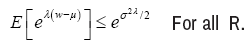
A random variable w with mean µ=E(w) is sub-Gaussian if there is a positive number σ such that

With this in mind, we given a third assumption, that’s (A3) The observation noise wi, i, ∈(1,. . . , n)is i.i.d. σ-sub-Gaussian variables. Before given the concrete corollary about Linear Kernel Regression, a Lemma about lower bounds for sub-Gaussian variables is needed.

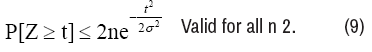
Lemma 2: Let (Zi)n i=1 be a sequence of zero-mean random variables, each sub Gaussian with parameter σ. (No independence assumptions are needed). Consider the lower bound of Z=maxi=1,. . . ,n X _i, we have

Corollary 3: Consider the S-sparse linear kernel regression model based on a noise vector w that assumption (A3) holds, and a deterministic design matrix X that satisfies assumptions (A3) and (A4). And the character Kernel satisfies the C-Column normalization condition: maxk=1, . . . , Suppose that we solve the Regular Linear Kernel Regression (3) with regularization parameter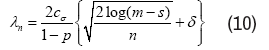

for some ∈ > 0. Then the optimal solution θˆ is unique with its support contained within S, and satisfies the l∞-error bound.

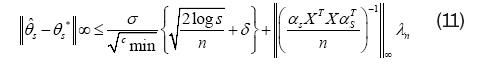
With probability at least

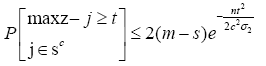
Proof: First, let us show that the given choice of λn(10) of the regularization parameter satisfies the bound(7) with high probability. It suffices to bound the maximum absolute value of the random variables

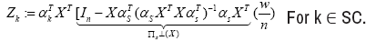
Since ΠSc (X) is an orthogonal projection matrix, we have

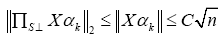
where the last inequality follows from the C-Column normalization condition. Therefore, each variable Z_j is sub-Gaussian with parameter at most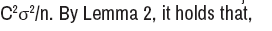

Transforming this to the |∞-norm form, we have

Substitute the choice of λn (10), we have 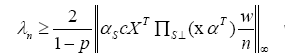with probability at least 1−2e− nδ2/2.

It remains to simplify the l∞-bound (8). Consider the random variables

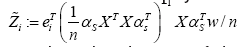
Since the elements of the vector w are i.i.d. σ- sub-Gaussian, the variable Z˜i is zero-mean and sub-Gaussian with parameter at most

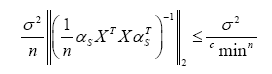
where we have used the eigenvalue condition (5). Consequently, for any δ > 0, we have

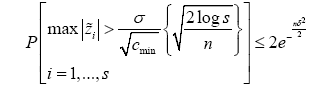
Then the claims follows from (1 − 2e;− nδ2/2)2 1-4e- nδ2/2

Upper to here, we have given the Kernel selection consistence conditions. By careful analysis of the original optimization problem (3), we find that the values of (θˆk)km=1 gradually diminish, as the penalize parameter λn is large enough. From condition (7), if the given parameter λn is too small, (7) condition is violated, we have no hope for excluding all fake Kernels. From part (d) of Theorem 1, the θˆi, i ∊ S, which cannot be zero, may be miscalculated as zero. In real world data detection, the choice of λ shall be carefully checked. Besides, Cross-validation methods are usually utilized for the decision of λn, or other improved methods [17].

Prediction error or risk assessment

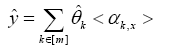
Another interesting twist is to do a risk assessment for all areas. Consider the Linear Kernel Regression Model (2). Given an estimation of ∈ˆ, the prediction of outbreaks yˆ is the superposition summation of the Kernels at the position of x, that’s

As this prediction yˆ is the linear combination of the Kernel functions, radiation effects of the true high-risk areas, at the point x, not just the number of the local outbreaks. We see yˆ as the risk assessment of the area x. Given a S- Sparse Linear Kernel Regression model, we devoted ourselves to bound on the mean-squared prediction error

Before giving the results, some more constraints about the design matrix, namely Restricted Eigenvalue (RE) condition shall be advertised here.

Definition 2

The matrix X satisfies the Restricted Eigenvalue (RE) condition over S with parameters (κ, γ) if

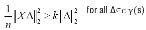
Here the subset Cγ(S)={Δ ∈ Rd|||ΔSc ||1 ≤ γ||ΔS||1}, is a collection of vectors. whose l1-norm off the support is dominated by the l1-norm on the support.

The Restricted Eigenvalue (RE) condition constructs a link between the

recovering error ||ˆθ−θ||2 and the prediction error ||XαT(ˆθ – θ*)||2. these set-ups, we give the bounds on prediction errors as follows

Theorem 4

(Prediction error bounds) Consider the Regular Linear Kernel Regression Optimization Problem(3) with a strictly positive regularization

parameter λn ≥2||αX^T w/n||∞. (a) Any optimal solution ˆθ satisfies the bound

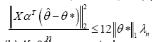
(b) If θ*is supported on a subset S of cardinality s, and the design matrix XαT satisfies the (κ; 3)-RE condition over S, then the optimal solution satisfies the bound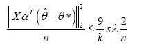

The proof of this prediction bounds can be seen in Appendix. Before that, let’s see what we are informed from the bounds. The two upper bounds are all related to λn. In order to reduce the forecast errors, a critical step is to reduce the regularization parameter λn.

Simulation studies

Consider a S-sparse Linear Kernel Regression model (2). Suppose each row xi of the design matrix X ∈ R^n×d is independently draw from a Gaussian distribution N(0, Id). And each αj of the candidates kernels α ∈ R^m×d is also i.i.d of Gaussian distribution N(0, I_d). The true support S is a subset of {1, • • • , m} uniformly distributed in [m]. The real parameter of θj*, j ∈ S is uniformly distributed on [−1,−0.1] ∪ [0.1, 1], and θj* = 0 for j ∈ Sc. Let the entries of the noise vector w follow i.i.d of a Gaussian distribution of N(0, 0.01).

Then the response variable Y is calculated by

Y=XαTθ+w.

Applied by the regular method of l1-norm, we are interested in the falseinclusion rate and consistency. False-inclusion rate is defined as,

False−inclusion=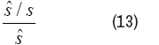

Where ŝ stands for the support of estimation θˆ. And the consistency between Ŝ and S, is given

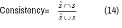
(F) and consistency (Con) under given levels of λn in Table 1. From Table 1, we known that the best result is F=0, which means no false inclusion and Con = 1, which means the estimation support Ŝ is identical with the true kernel support S. For λn that’s not too small, the no false inclusion holds. And the consistence grows up and down, as λn increases. The consistence holds for a long time as we increase the value of λn, which means that for a long period, the support of θˆ makes no changes. And this information will be useful for empirical selection of the regularization parameter λn.

Further, we find that the sample dimension has an important relationship with the consistency. We calculated the average consistency under different dimensions of d ∈ [40, 100, 200, 300, and 500]. The average is the result of 100 replicates, where the λn is chosen according to maximizing consistence. From the results in Table 2, it’s easy to find that as the dimension increases, the average consistency increases steadily. As the number of candidate Kernels increase, picking out exactly the true supports becomes more difficult. From here, we get the revelation that increasing the dimension of the data is of great significance to correctly pick out the Kernels. And reducing the number of candidate kernels is also useful for reducing false inclusion rates and improving consistency.

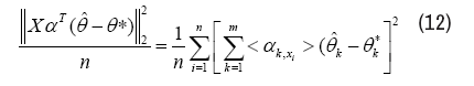
Finally, we care about the changing law of the prediction error, by adding tests check. We draw the test data-set by choosing a test design matrix X^test ∈ R^{T ×d}, with each row xi test follows a Gaussian distribution N (0,I^d). And the test response variable Y ^test is calculated by

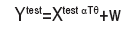
The prediction error is calculated by equation (12). The curves of prediction error along λn were plotted in Figure 1 under given levels of s [5, 10, 15, 20], which stands for the number of true Kernels. Here n=1000, m=1000, d=500, T=500, where T stands for the size of test data-set. From the results of the Figure 1, the prediction error grows as λn goes beyond some fixed point. And for the different levels of s, the prediction error grows proportional to s, which is coincident with the result from part (b) of Theorem 4.

Discussion

High-risk areas selection and risk assessment of COVID-19

In this section, we try to explore high-risk areas of COVID-19 with the outbreaks of COVID-19, provided by https://fy.onesight.com/. This data includes the number of confirmed cases in each country since the outbreak of COVID-19. As the data collection deadline is September 2021, we had to collect the relevant covariates of each country up to that point in time. First, we collected the coordinates of the capital of each country, from the latitude βt and longitude βg, by

{x=cos(βt)cos(βg), y=cos(βt) sin(βg), z=sin(βt)}

As mentioned earlier, the COVID-19 now spreads mainly in the form of person-to-person spread. So in the second part of date collection, the variables of population transmission were collected, including population, population density per square kilometer, population birth rate and Gross Domestic Product (GDP), which concerns the activity of each country.

And in the third part of the data collection, the history of death toll of COVID-19 by weeks is also collected from https://www.kaggle.com/tarunkr/ COVID-19-case-study-analysis-viz-comparisons from January 2020 to September 2021. In summary, we collected outbreaks and associated covariates of 114 dimensions for 189 countries.

The first concern is the selection of high-risk areas. We make all 189 countries or regions be candidates of Kernels. Before the regular Linear Kernel Regression model being implemented, a normalize scale of data set is employed, as follows

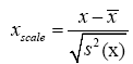
Here, x¯ stands for sample mean of x and S2(x) stands for sample covariates, S2(x)=1 Σn (xi − x¯) 2. Given several levels of λn, the Kernel areas selected were given in Table 3. In the table, high-risk areas are countries whose coefficients are positive. Purification areas are countries, whose coefficients are negative.

Another meaningful task is to carry out a risk assessment of all candidate areas. Given λn=0.5, we made a risk assessment for all 189 countries or areas. The risk is calculated by

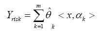
As all variables of covariates were scaled with zero-mean and standard deviation S2(x)=1, including the number of outbreaks. So the risk Yrisk of each area takes values around 0. For high-risk areas, the response Yrisk is also large. In particularly, the assessment results are presented in Table 4, 5. From the risk assessment table, we see that Brazil, United Kingdom and Russia are of high risk in risk assessment program. While in purification areas selection, they are viewed as purification areas. The reason lies in the those areas are close in ”distance” with high-risk areas and actually they are victims. They are surrounded by the true COVID-19 emission sources. The relation between high-risk selections with risk assessment is that high-risk selection is finding the causes or emission sources and risk assessment is the presentation of spreading of COVID-19. For some areas that are judged to be of great risk assessment, they are likely to be innocent and may be purification areas. With Kernel selection of high-risk areas, only then can we decide whether an area is a true source of transmission, not just by risk assessment.

Conclusion

In this paper, we considered the condition of Kernel selection consistence, in Regular Linear Kernel Regression Model with l1-norm. And bounds on the prediction error of RLKR are also given with mild conditions. Then we applied the RLKR to high-risk selection and risk assessment for COVID-19, in a view point of area-to-area spreading mode. In the simulation of random design matrix, we explored the F alse−inclusion and Consistency under different levels of λn and the number m of candidate kernels. The prediction error bounds were also checked with a no-wise result. In real world data of COVID-19, the risk assessments of 189 numbers of countries or areas were given. We believe this will provide valid advices on traveling.

Acknowledgement

Our thanks go to Professor Bo Li for stimulating this research. Our research is supported by NSF of China (Grant No. 61877023) and the Fundamental Research Funds for the Central Universities (Grant No. CCNU19TD009).

References

1. Fauci Anthony S, H. Clifford Lane and Robert R. Redfield. “Covid-19 - Navigating the Uncharted”. N Engl J Med 382(2020):1268-1269.

   [Crossref] [Google Scholar] [Pubmed]

2. Yuki Koichi, Miho Fujiogi and Sophia Koutsogiannaki. “Covid-19 Pathophysiology: A Review”. Clin Immunol 215(2020):108427.

   [Crossref] [Google Scholar]

3. John H Beigel, Kay M. Tomashek, Lori E. Dodd and Aneesh K Mehta, et al. “Remdesivir for the Treatment of Covid-19 - Final Report”. N Engl J Med 383(2020):992-994.

   [Crossref] [Google Scholar] [Pubmed]

4. Felsenstein Susanna, Jenny A.Herbert, Paul S.McNamara and Christian M.Hedrich. “Covid-19: Immunology and Treatment Options”. Clin Immunol 215(2020):108448

   [Crossref] [Google Scholar] [Pubmed]

5. Lotfi Melika, Michael R.Hamblin and NimaRezaei. “Covid-19: Transmission, Prevention, and Potential Therapeutic Opportunities”. Cli. Chim Acta 508(2020):254-266.

   [Crossref] [Google Scholar] [Pubmed]

6. Ndairou Faical, Ivan Area, Juan J.Nieto and Delfim F.M.Torres. “Mathematical Modeling of Covid-19 Transmission Dynamics with a Case Study of Wuhan”. Chaos Soli 135 (2020):109846.

   [Crossref] [Google Scholar]

7. Gostic Katelyn, Ana CR Gomez, Riley O Mummah and Adam J Kucharski et al. “Estimated Effectiveness of Symptom and Risk Screening to Prevent the Spread of Covid-19”. Elife 9(2020):55570.

   [Crossref] [Google Scholar]

8. Bleier Benjamin S, Murugappan Ramanathan and Andrew P. Lane. “Covid-19 Vaccines may not Prevent Nasal Sars-Cov-2 Infection and Asymptomatic Transmission”. Otolaryngology. J OTOLARYNGOL-HEAD N 164(2021):305-307.

   [Crossref] [Google Scholar]

9. Osborne Michael R, Brett Presnell and Berwin A. Turlach. “On the Lasso and its Dual”. J Comput Graph Stat 9(2000):319-337.

   [Crossref] [Google Scholar]

10. Zhao Peng and Bin Yu. “On Model Selection Consistency of Lasso”. J Mach Learn Res 7(2006):2541-2563.

    [Google Scholar]

11. Hastie Trevor, Andrea Montanari, Saharon Rosset and Ryan J. Tibshirani. “Surprises in High-Dimensional Ridgeless Least Squares Interpolation”.1-6(2020).

    [Crossref] [Google Scholar]

12. Bartlett Peter L, Philip M. Long, Gabor Lugosi and Alexander Tsigler. “Benign Overfitting in Linear regression”. Proceedings of the National Academy of Sciences 117(2020):30063-30070.

    [Crossref] [Google Scholar]

13. Tuo Rui, Yan Wang and C. F. Jeff Wu.  “On the Improved Rates of Convergence for Matérn-type Kernel Ridge Regression, with Application to Calibration of Computer Models”. Int J Uncertain Quantif 8(2020):1522-1547.

    [Crossref] [Google Scholar]

14. Fanghui Liu, Zhenyu Liao and Johan A.K. Suykens. “Kernel Regression in High Dimensions: Refined Analysis beyond Double Descent”. Proceedings of Machine Learning Research. 130(2021):649-657.

    [Crossref] [Google Scholar]

15. Lorin Crawford, Kris C. Wood, Xiang Zhou and Sayan Mukherjee. “Bayesian Approximate Kernel Regression with Variable Selection”. J Am Stat Assoc 113(2018):1710-1721.

    [Croosref] [Google Scholar]

16. Liang Tengyuan and Alexander Rakhlin. “Just Interpolate: Kernel "Ridgeless" Regression can Generalize”. Ann Stat 48(2020):1329-1347.

    [Crossref] [Google Scholar]

17. Braga Igor and Maria Carolina Monard. “Improving the Kernel Regularized Least Squares Method for Small-Sample Regression”. Neurocomputing 163(2015):106-114.

    [Crossref] [Google Scholar]