Trend of Tobacco Production, Its Cost of Raw Materials, Amount of Product, Sales Value and Tax Paid in Ethiopia; Application of Multivariate Time Series Analysis

Awoke Seyoum Tegegne^1* and Wosenie Gebireamanuel Hailu^2
*Correspondence: Awoke Seyoum Tegegne, Department of Statistics, Bahir Dar University, Bahir Dar, Ethiopia, Email:

Keywords

Tobacco • Vector error correction model • Co-integration • Granger causality • Impulse • Response • Forecasting

Abbreviation

AD: Anno Domini; ADF: Augmented Dickey-Fuller; AIC: Akaike Information Criteria; AR: Autoregressive; BC: Before Crist; BIC: Schwarz-Bayesian Information Criteria; CCM: Cross Correlation Matrix; CI: Confidence Interval; CV: Coefficient of Variation; EFMHACA: Ethiopian Food; Medicine and Health Care Administration and Control Authority; ETB: Ethiopian Birr; FCTC: Framework Convention on Tobacco Control; FEVD: Forecast Error Variance Decomposition; GATS: Global Adult Tobacco Survey; HQIC: Hannan-Quinn Information Criteria; IID: Identically and Independently Distributed; IRF: Impulse Response Function; LM: Lagrange Multiplier; MA: Moving Average; MAE:

Introduction

Different countries use tobacco as a source of income and play a vital financial role. For instance, in Indonesia tobacco provides a significant contribution as a source of income for farmers and provides employment [1]. Tanzanian tobacco has a significant contribution to GDP, employment, and provides large exercise tax revenue to the government [2]. Also in Ethiopia it used as source of tax revenue and employment opportunity [3]. Tobacco provides significant economic benefits to countries around the world [4]. The tobacco industry occupies an important position in China’s economic development [5]. Tobacco production can bring huge economic benefits to society and the government [6].

Local production of tobacco products and import trade constitute the main sources of tobacco products. Ethiopia has only one tobacco manufacturing industry partially owned by the government. Chemical ingredients of tobacco products should be announced to EFMHACA so that appropriate feedback would be given to the manufacturers and importers. Many Ethiopians are employed in the tobacco processing factory and its’ farm [7]. National tobacco enterprise (Ethiopia) is a manufacturer and distributor of tobacco products. The company's tobacco products include cigarettes, cigars, cigarillos, and pipe and water pipe tobaccos, enabling customers to enjoy quality tobacco products.

Ethiopia gets 30% of its tobacco leaf supply from four National Tobacco Enterprise owned farms in different parts of the country. These are namely, Shewarobit in the Amhara regional state and three farms in Hawasa, Wolayeta and Belate in the SNNPR. The remaining 70% obtained through importation [8]. Tobacco leaf is the crucial constituent in cigarettes and other tobacco products [9].

Tobacco use is the leading cause of preventable death in worldwide. In Ethiopia from 2016 Global Adult Tobacco Survey (GATS) data shows that 3.7% of individuals aged ≥ 15 years (6.2% men and 1.2% women) currently smoked tobacco products, and 29.3% and 12.6% of adults were exposed to secondhand smoker at the workplace and home, respectively. Some of the common impacts of tobacco use include direct expenses to purchase tobacco products, medical cost for treating tobacco-related illnesses and lower workplace [10]. Tobacco cultivation poses a significantly high environmental cost that causes a net loss to society [11]. Cigarette is made up of tobacco, paper and additives. Tobacco plant is open to absorb and accumulate heavy metal species from the soil into its leaves [7]. Heavy metals such as mercury, cadmium and lead is a serious growing problem throughout the world [12].

Ethiopia was one of the many countries that signed the convention to ratify the WHO FCTC early in 2004. However, the country’s tobacco industry used as ‘a source of tax revenue and employment opportunity’ have resulted in major obstacle to ratifying and implementing WHO FCTC. In early 2014, Ethiopia took a significant step toward tobacco control and gave the mandate for implementing the WHO FCTC to the Ethiopian Food, Medicine and Healthcare Administration and Control Authority (FMHACA) [13]. The WHO global report on prevalence of tobacco use (2000-2025) contains country specific information and projections that will provide government, policy makers and regulators valuable information. The report provides a comprehensive analysis of trends and projections of tobacco use internationally toward the global voluntary target of 30% relative reduction in tobacco use by 2025 [14]. Ethiopia's government passed an anti-tobacco notice in 2015, which includes measures governing tobacco consumption, advertising, packaging, and labeling [15]. Also the strategic plan of 2018-2020 is to eliminate all forms of illegal tobacco product trade by adopting, developing, and implementing effective legislative, executive and administrative measures [16].

Tobacco has various negative impacts on the societies. These impacts are very series for smokers and secondhand smoker especially on their health and social life. Tobacco has different economic, social, health and other problems to the societies [17,18]. The Ethiopian government wants to decrease and control tobacco usage and reduce it by 30% in 2025 which is adopted from the WHO plan. Identifying the association or relationship between raw material costs, amount of tobacco production, total sales value and tax paid about tobacco product is important to achieve the government tobacco usage reduction plan. So there is a limitation in Ethiopia on the relationships among tobacco production, total sales value and tax paid about tobacco product.

Different studies revealed that there is a relationships or association among the cost of raw materials, amount of production, sales and tax paid for tobacco product [19,20]. However, these studies used cross-sectional time-series data about cigarette excise tax has effect on revenue, cigarette price and consumption, sales of tobacco product using logistic regression and time series analysis, impact of tobacco sale on employment and tax using macroeconomic models, tobacco production and tobacco raw material.

But these researches also tried to investigate the relationship between two of variables rather than all events happened from production to end results four variables together. In addition to this, as far as our knowledge is concerned, there are no researches on raw material cost, amount of tobacco production, total sales value and tax paid in Ethiopia using multivariate time series model. Showing all the relation between such events might be important for policy implication and reach to right decision at country level.

Therefore, to reduce the tobacco usage and its impact on the societies, assessing the association between raw materials cost, production, sales and tax paid for tobacco product is very important. After identifying the relationship based on the study result, policy makers and policy executors can set and enforce the policy to minimize tobacco usage, diseases and deaths come from tobacco. Hence, the main objective of the current study was to investigate to process of tobacco production, its cost of raw materials, amount of production and sales value and tax paid in Ethiopia.

Materials and Methods

Study area

Ethiopia has only one state owned national tobacco manufacturing company which is established in 1942 and which is located in Addis Ababa. Addis Ababa is the capital city of Ethiopia and headquarters of African union. Also it is the largest city in Ethiopia. Ethiopia is the most populous country out of the horn of African countries and the second most populous country in Africa next to Nigeria. According to World Bank estimation in 2021 Ethiopia has 120,283,026 total populations.

Data source

The data was taken from Ethiopian statistics service which is an agency of the government of Ethiopia that designated to provide all surveys and censuses for the country used to monitor economic and social growth, as well as to act as an official training center. This agency conducted different surveys in each year. Among the yearly data that collected by this agency is from manufacturing industry. National Tobacco Enterprise (Ethiopia) share company is one of the large and medium manufacturing industries in Ethiopia and central statistical agency collect annual data from this company in each year.

In this study, the data was the secondary data on annual raw material cost, amount of annual production, total sale value and tax paid which was obtained from new name Ethiopian statistics service (the former name was Central Statistical Agency (CSA)) over the year starting from the year 1996 to 2018 because of the data availability.

Variable of the study

Under this study variables of interest include total annual raw materials cost, the total annual production amount, total annual production sales value, and tax paid are used as endogenous variable for tobacco production. The lags of all endogenous variables were used as explanatory or exogenous variables.

The variables under study and their abbreviations are cost of raw materials (rcost, in Ethiopian birr), total product (prod in number of sticks), total sales value (Ethiopian birr), tax paid (Tax in Ethiopian birr).

Descriptive analysis

It used to summarize or describe the characteristics of the study variables such as count, average, standard deviation, coefficient of variation, minimum, maximum, range and so on. The data or the series was summarized by using tabular data presentation.

Multivariate time series statistical method

The study employed multivariate time series analysis such that vector autoregressive model especially vector error correction model due to the presence of cointegration relation. A time series is a sequence of observations obtained through measurements often recorded at equally spaced intervals. Multivariate processes arise when several associated time series processes are observed simultaneously (or concurrently) over time and it used to describe the interactions and co-movements among a group of time series variables.

The goals of jointly assessing and modeling the series are to better understand the dynamic relationships between the series over time and to improve the accuracy of forecasts for individual series.

The length of time series can vary and many models require at least 50 observations for accurate estimation for univariate time series modeling but generally at least 20 observations long. At the very minimum, a time series should be long enough to capture the phenomena of interest. According to Liu, et al. the length restriction to N>P, which makes it possible to model many short time series models where N is the number of observations over time and p is the maximum lag or order. In multivariate time series analysis very small lengths are permitted.

To investigate the dynamic relationship between the series over, the stationary stochastic process was considered. In addition, the Augmented Dickey-Fuller (ADF) unit root test, tests of stationarity, data transformation processes and trend and seasonal adjustments were conducted.

Model adjustments considering, Vector Autoregressive Model (VAR), order specification for VAR, estimation of parameters for VAR and stability of VAR process were tested and investigated.

Model diagnostic checking: In times series model, checking the validity and reliability of the model is very essential before making forecast for the future some series. There are different diagnostic tests those are useful to check the validity of assumption and properties. Model adequacy checking were conducted using.

Test for residual autocorrelation: Residual analysis is a critical step in the development of empirical time series model. When assessing the model’s adequacy, one typically looks for the presence of residual autocorrelation. The Breusch-Godfrey Lagrange Multiplier (LM) test and Portmanteau test are the two common types of residual autocorrelation tests.

Autocorrelation LM test: In the VAR(p) process Lagrange multiplier test can use to identify the residual autocorrelation. For the VAR model

The most widely used and well established test for stationarity in time series is the ADF test. This test used to test whether a unit root is present in an autoregressive model or not.

Consider an autoregressive order one process given by

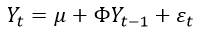
where, Y_t is the variable of interest and ε_t is the error term which is assumed white noise. If a unit root is present (that is, if =1), then the model would be non-stationary. After subtracting Y_t-1 from both sides of the equation (4) then the model can be written as:

In ADF, testing for a unit root in the above model is equivalent to testing:

H₀: π=0 (the series is not stationary) vs. H1: π<0 (the series is stationary)

The test statistic is given by tπ=πse(π) where π is the estimate of π and se(π) is the standard error of the estimate.

The ADF test constructs a parametric correction for higher-order correlation by assuming that the series follows an AR (p) process and adding lagged difference terms of the dependent variable. If the series are serially correlated, then εt can be expressed as:

Phillips and Perron (PP) unit root tests: The statistic proposed by Phillips and Perron arise from their considerations of the limiting distributions of the various Dickey-Fuller statistics when the assumption that is an iid process is relaxed. The PP test can correct for any serial correlation and heteroscedasticity in the errors εt of the test regression by directly modifying the Dickey-Fuller test statistic. The PP test estimates the non-augmented ADF test in equation (5) and establishes the t ratio of the π coefficient so that the serial correlation does not affect the asymptotic distribution of the test statistic. The PP test is based on the statistic:

Trend and seasonal adjustments: A time series that exhibits a trend is a non-stationary time series. Modeling and forecasting of such a time series is greatly simplified if we can eliminate the trend. One way to do this is differencing. That is, applying the difference operator to the original time series to obtain a new time series, say,

X_t=∇_yt=y_t-y_t-1 Where, ∇ is the (backward) difference operator

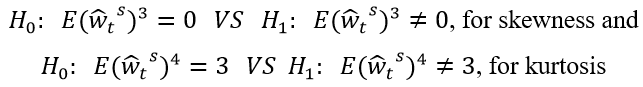
Testing normality of the residuals: Multivariate generalization of the test statistic T/6 ((S²+(k-3)²)/4) use to test multivariate normality of the residual wt where T is number of observations, S is sample skewness and k is sample kurtosis. The statistic uses the wt (3^rd and 4^th) moment i.e., skewness and kurtosis of the multivariate normal distribution. The hypothesis is:

Forecasting: Forecasting is the second main objective of time series analysis for a certain h ≥ 1 step ahead. For this study forecasting is for the vector autoregressive model can be executed in a recursive manner. Forecasting for vector time series model is similar to univariate autoregressive time series model forecasting or it is a generalization of univariate time series model.

To forecast using VAR model, number of variables (let n) and number of lag (let p) in the system is very important. The number of coefficients to be estimated in the VAR is equal to n+pn² in the system or 1+pn for each equation. For example, if there are four variables and the lag is three, there are 4+3 × 42=52 coefficients (total coefficient in the system). Also there are 1+3 × 4=13 coefficients in one equation.

Measure of forecasting accuracy: In time series analysis measuring the goodness or appropriateness of forecasting is very important. Let define Y_t is the observed or actual value for period t and Z_t is the forecast value for a certain period, the error becomes ε_t=Y_t-Z_t.

Results

Descriptive statistics

The descriptive statistics of the current study is indicated in Table 1. Table 1 indicates that the average, the company produces annually 712.4 million tobacco sticks, the annual raw material cost was around 603.02 million birr, and the sale value becomes around 1.58 billion birr with the paid tax 188 million birr. The descriptive statistics shows that the product of tobacco increased from its minimum value 699303 sticks in 2002 to its maximum product value 3658964298 in 2017. Similarly, the raw material cost increased from its minimum value 47536306 birr in 2005 to its maximum cost value 2520553990 birr in 2013. Also the total sale value of tobacco product increased from its minimum value 243486289 birr in 1996 to its maximum value 5457776082 birr in 2016. The tobacco tax increases from minimum value 43885615 birr in 2000 to its maximum value 584879841 birr in 2016.

Table 1. Descriptive statistics summary.

The kurtosis values of the series are more than 3 except sale value and these indicate that the series are leptokurtic (sharp toped) but sale value is around 3 and it shows mesocratic (the series is normally distributed).

Stationarity test: There are two ways to identify the stationarity of the series. Those are graphical method and unit root test. Stationary series show the mean, variance, covariance does not vary with time or they are not the function of time. In time series analysis checking stationarity is a preliminary activity before attempting fitting model.

Time plot: Time series plots are commonly regarded as the best choice for visualizing time series data by representing temporal changes of values using up and down slopes, they enable us to clearly identify trends and other patterns.

The time plot for current investigation is indicated in Figure 1. Figure 1 indicates that there exist upward trends in all series but up to 2007 the series seem to steady. The raw material cost seems decreasing after around 2016. The plot shows the series have a comovement and it shows that they have common characteristics. The trend suggests the mean is not constant and it implies a nonstationarity behavior of the series. Generally, the series have an upward increasing trend.

Figure 1. Time series plot for the study variables at level.

Unit root tests: According to the above time plot, the series exhibits non-stationary behavior at levels. In addition to time series plot test of stationarity it is better to apply different unit root testing such as Augmented Dickey Fuller (ADF) and Phillips Perron (PP) because the test provides more evidence than the graphical way.

Both tests have similar hypothesis that is on the null hypothesis states that the variable under investigation has a unit root or nonstationary series versus the alternative hypothesis states that it does not has unit root. The decision rule is reject the null hypothesis if the ADF/PP test t-statistic value exceeds (in absolute value) the critical value at 5% level of significance reject the null hypothesis. These results are presented in Table 2 below using Eviews-10.

Under this study the test found to have unit root or non-stationary at level both without trend and with trend for the series log(prod), log(rcost), log(sale) and log(tax) at 5% level of significance.

Series: log (prod) log(rcost) log(sale) log(tax)

Table 2. Group unit root summary at level with constant.

From the Table 2, we can conclude that assuming both the common unit root process and individual unit root process the null hypothesis does not rejected and this implies there is a unit root or a non-stationarity in level with constant. To clarify more test individual series as follow and the result displayed in Table 3.

Table 3. Unit roots test results (At levels).

Table 3 indicates that both of the augmented dickey fuller test and Phillip Perron test Statistic greater than the 5% significant level critical value hence unit root is existing in level with constant, and trend with constant at level for individual series.

The results in Table 4 indicate that the null hypothesis of unit root is rejected for the first differences of the four variables with intercept using ADF and PP test. This implies that the four variables or series are integrated of order one. Therefore, the ADF and PP test based on Tables 3 and 4 shows that all series are non-stationary at levels and stationary at the first differences respectively. Co-integration analysis is thus feasible for those series and would be used.

Vector Autoregressive (VAR) model specification: The VAR model is a stochastic process model that is used to reflect the linear interdependencies between several time series. In this model all variables are enter in the same way: each variable has an equation explaining its evolution based on its own lagged values, the lagged values of the other variables, and an error term.

Under this study the variables are transformed by using natural logarithm. The reason for utilizing log-transformed data in time series regressions comes from the normality assumption and tries to reduce the negative impact of heteroscedasticity and skewness in the level data on estimation and testing results.

Cross Correlation Matrix (CCM): The degree of correlation between different time series variables is described by cross correlation. Cross-correlation is used to examine whether a change in one-time series may influence a change in another time series. When the value of one variable increases, the value of the corresponding variable increases as well, or both variables decrease concurrently for associated variables.

Table 4. Unit roots test results (At their first difference).

Based on Table 5 below, there exists high positive cross-correlation between log(prod), log(rcost), log(sale) and log(tax) up to two order pre-determined or lagged value; log(rcost) and log(tax) with the others highly correlated up to third lagged value but after lag three up to five all series have less positive cross correlation value and after five some series have negative correlation value.

Table 5. The correlation matrix of the study variables.

VAR order specification: An important aspect of empirical research based on the Vector Autoregressive (VAR) model is the choice of the lag order, since all inferences in this model depend on the correct model specification. Determination of optimal lag order for the VAR model is performed using the Akaike Information Criterion (AIC), Schwarz Bayesian Information Criterion (SBIC) and Hannan-Quinn Information Criterion (HQIC). The lag with a minimum criterion value is selected as an optimum lag length for the model (Table 6).

Table 6. VAR lag order selection criteria result.

Lag exclusion test

The Wald lag exclusion test was used to check whether the selected lag is optimal or not jointly. This test was carried out for the confirmation for suitability of each lag selected by the four information criteria. The result in this study indicates that third lag was the optimal lag for VAR model at 5 percent level of significance. For each lag the Chi-square (Wald statistic) of all series were reported separately and jointly. Hence, VAR (3) was found suitable for the data set and hence could be adopted.

Parameters estimation for the VAR (3) model: After identifying the optimal lag length, the next step was estimating the VAR parameters. Parameter estimation was conducted using maximum likely hood estimation technique. In parameter estimation approach four questions were considered.

In the first equation, product was considered as a dependent variable and the rest as predictor. In the second equation, a raw material cost as dependent and the rest as predictors. In the third equation, sale was considered as dependent and the rest were considered as predictors. In the fourth equation, tax was considered as dependent and the rest as predictors.

The result in the first equation is interpreted as follows for a onebirr increase in first and third period lagged values or pre-determined values of tax paid and the second pre-determined value of tobacco sale in logarithm form while keeping other factors constant then results of product in logarithm for the current period is increased by 0.96 pieces, 1.12 pieces and 1.81 pieces respectively. Also a one-birr increase in the third period lagged value of product, the product in the current period was decreased by 0.40 pieces. Hence, in this equation, sale and tax has a positive significant effect and the product as a negative effect by itself in the short run during the study period. The R-square value for product equation is 0.9463, which indicates that 94.63% of the variation of future product was explained by the variables included.

The result in the second equation (raw material cost as dependent variable) indicates that for a one-birr increase in the first, second and third period lagged values or pre-determined values of raw material cost, in the second and third period lagged value of tax in logarithm form while keeping other factors constant, results of raw material cost in logarithm for the current period is increased by 0.86 birr, 0.38 birr, 0.46 birr, 1.12 birr and 2.08 birr respectively. For a one stick increase in the second and third period lagged value of product, the raw material cost for the current period was increased by 0.46 birr and 0.32 birr respectively. A one-birr increase in the first, second and third pre-determined lagged value for sale the result of the raw material cost for the current period was decreased by 1.03 birr, 1.85 birr and 1.52 birr respectively. The R-square value is 0.9177, this indicate that 91.77% of the variation of future raw material cost was explained by the included variables.

The result in the third equation (sale as dependent variable) indicates that product, raw material cost and tax paid had positive effect for sale value at the first, second and third pre-determined lagged value but sale value had negative effect for itself in the first, second and third pre-determined lagged value. For one-piece increase of tobacco product at the first, second and third predetermined lagged value, the sale value for the current period was increased by 0.08 birr, 0.27 birr and 0.18 birr respectively. Also for one-birr increase in raw material cost at the first, second and third pre-determined lagged value, the sale value for the current period was increased by 0.33 birr, 0.40 birr and 0.35 birr respectively. A one-birr increase in sale value at the first, second and third predetermined lagged value, the sale value for the current period was decreased by 1.53 birr, 1.16 birr and 0.65 birr respectively. A one-birr increase of tax paid at the first, second and third pre-determined lagged value, the sale value for the current period was increased by 1.04 birr, 0.81 birr and 1.17 birr respectively. The R-square value is 0.9893, this indicate that 98.93% of the variation of the future sale value is explained by the variables included.

The result in the fourth equation (tax as dependent variable) indicates that, for one-birr increase in raw material cost at the first pre-determined lagged valued of raw material cost, the tax paid for the current period was decreased by 0.13 birr. For one-birr increase in raw material cost at the second and third lagged value, the tax paid for the current period was increased by 0.38 birr and 0.40 birr respectively, for one-birr increase at the first, second and third lagged value of the sale value, the expected tax paid for the current period was decreased by 0.69 birr, 1.56 birr and 0.88 birr respectively. For birr increase in tax paid at the first, second and third lagged value, the expected value of tax paid for the current period was increased by 0.87 birr, 0.45 birr and 1.29 birr respectively. The R-square value in this case was 0.9377, which indicates that 93.77% of the variation in the future value of tax paid was explained by the variables included.

Model adequacy checking: After fitting the model, diagnostic testing is required before making forecasting in time series analysis. Under this study roots of characteristic polynomial stability condition tests for model stability test, Breusch-Godfrey serial correlation LM test, Breusch-Pagan-Godfrey of Heteroscedasticity test, and Jarque-Bera test for normality tests were used to check the adequacies of VECM model.

Stability analysis of the VEC model: If the dots are outside the circle, the model is not stationary, and the impulse response result is invalid. But the results from roots of characteristic polynomial stability condition in Figure 2 showed that the VECM model satisfies stability conditions because all the roots lie inside the unit circle.

Figure 2. Inverse root of AR characteristic polynomial graph for VECM.

Test of residual autocorrelation: Here the Lagrange Multiplier (LM) and Portmanteau Q-statistic test were applied to check presence or absence of residual serial correlation or autocorrelation/lagged correlation/. The result revealed that the null hypothesis of no serial autocorrelation was accepted for the Godfrey LM test for all lags undertaken.

Residual normality test: To test the residuals normality, multivariate version of the Jarque Bera tests were applied. It compares skewness and kurtosis to those from a normal distribution. The two hypotheses are the null hypothesis claims that residuals are multivariate normally distributed, while the alternative hypothesis states that residuals are not normally distributed in multivariate space. Since the p-value greater than 0.05 in 5% significance level for the Jarque-Bera test of normality, skewness and kurtosis tests indicates the null hypothesis (H₀) is not rejected for all residuals which imply that the residuals are all normal.

Forecasting: Time series forecasting is using available observations from a time series to forecast its value at some future time t+h. It is the second major objective of time series analysis. Based on the given data the study examined the forecasting accuracy of VEC (2) model and then makes a forecast from 2019 to 2025 for seven years ahead for tobacco product, raw material cost, sale value and tax paid.

Measure or evaluation of forecasting accuracy: There are most common evaluation mechanism to assess the forecasting performance such as Mean Square Error (MSE), Root Mean Square Error (RMSE), Mean Absolute Error (MAE) and Theil U statistics. The lower values of MSE, RMSE, MAE and Theil statistics implies the model is good to forecast the series value.

Based on Table 7, the value of RMSE, MAE, MAPE and Theil are very small and these imply the model is efficient and reliable to forecast the series value. The mean absolute percentage error shows the average percentage variation of predicted values from the actual value. The MAPE value for log(prod), log(rcost), log(sale) and log (tax) are 3.34%, 2.14%, 0.46% and 0.76% and this implies the predictions are on the average 3.34%, 2.14%, 0.46% and 0.76% away from the actual value for product, raw material cost, sale value and tax paid respectively. All are less than 5% and these are indicator of good forecasting accuracy.

Table 7. Forecasting evaluation table.

Also the Theil inequality coefficients U are very small and approach to zero. These also imply the model is efficient and reliable to forecast the series value for h steps ahead. In addition to this Figure 3 shows the actual values and the forecast values are much closed to each other. So this also suggests the presence of minimum difference or gap between the forecasted values and actual values leads to less error.

Figure 3. Actual, fitted and residual plot for LOG (PROD).

Out of sample forecasting analysis: Since the VEC (2) model is good to forecast some future value of the series, outside or h steps ahead forecasting was done. Table 8 shows the result of seven steps ahead forecasts using VEC (2) model.

Table 8. Seven years forecast values from the VEC Model.

From Table 9 the annual tobacco product increase from three hundred million pies in 2019 to five billion pieces in 2025 and also the annual raw material cost also shows increment from 2019 to 2025 but there is a little fluctuation. The annual sale value and tax paid have increments as a whole but there exist obvious increase and decrease values in some period.

Table 9. Out of sample forecasting VECM results.

Figure 4 also shows similar result from the above Table 8 value. Figure 4 tells us increasing value with some fluctuated values. But it gives information that the whole series tends to increasing trend.

Figure 4. Graph for the seven years’ future logarithmic forecasted values.

Discussion

The current study tried to investigate the relationship between tobacco product, raw material cost, sale value and tax paid in Ethiopia using time series data using the time series data from 1996 to 2018 collected by Ethiopian statistics service from national tobacco enterprise. The Ethiopian tobacco production enterprise is one of the large and medium manufacturing industry in the country. The study based on special vector autoregression model that is vector error correction analysis suggested that product can have a significant positive effect on tobacco product. This finding was supported by the research of Bangara BC using other model Cobb Douglas production function to estimate tobacco production and the research of Porru S, et al. suggested that cigarette production rises year after year in Indonesia by producing much billion cigarette sticks. More over in this study indicates that as increasing one stick at the first and second lagged tobacco product leads to increase the tobacco product by 0.5675 stick and 0.3982 stick in differenced logarithm form in the short run relationship. In the long run relationship tax paid has negative effect on product. For one-birr increase in tax leads to decrease the product by 0.1858 stick in logarithm based on the first cointegration equation.

From this study the result of VECM indicate that raw material cost negatively affected by tobacco product in the short run relationship and this result contradict with the finding of Nwogwugwu UC, et al. this suggest that increasing cigarette production leads to increase the raw material cost this may be due to difference of size of observation and model but in this study raw material cost and product have positive relationship in long run equilibrium and supported by Sen A, et al. result.

This study revealed that product has positive relationship with sale value from the long run equilibrium and has native relationship in short run equilibrium. The finding of Mayer T also suggested that producing more product leads to increase the total revenue or sale value. In this study the result shows sale value has negative relationship with tax. Tobacco tax increments can result in decrement of sale value. Because increasing tobacco tax leads to increase the retail or sale price on tobacco product and this decrease the total sale value. This supported by Alshirah AA.

From this study sale value positively affected by cigarette sale at first and second lagged value in the short run relationship. This study also supported by Cotti C, et al. that cigarette sales are positively affected by cigarette sale. Guizhou Province's overall cigarette sales have increased year after year. The reduction in flue-cured cigarette production may be because of the enforcement of the planned fluecured cigarette production reduction by the nation. Moreover, China’s cigarette consumption tax was adjusted and affects cigarette consumption.

The causal relationship between cigarette sales and economic factors are verified via Granger's causality test. Here in this study also VEC Granger causality test identify sale value has one directional relationship with product and bi-direction with raw material cost and tax.

From this study the long run relationship shows that tax has positive relationship with product. Decreasing the amount of product leads to decreasing tax paid in the long run but they have negative relationship in short run. The AL-Qudah, AM finding result also show that eradication of tobacco products would have reduced Michigan's tax revenues. Moreover, Hiscock R., et al. had also found the impact of a tax increase that leads the smokers switch to cheaper brands and minimize tobacco usage.

Also the VEC result shows more of the variables affect negatively for the other variables that nominated as dependent variable especially in the short run relationship with the differenced logarithm form. Basically tax has negative on sale value and this leads to decrement of sale value and has negative impact for cigarette development economy for the company.

Conclusion

The current study indicates that the tobacco product is significantly affected by its own first and second lagged values only. Raw material cost is positively affected by sale value at both first and second lagged values while the remaining series such as product, raw material cost and tax paid have negative effect on raw material cost at first and second lagged values. Sale value is positively affected only by its own first and second lagged values and it is negatively affected by product, raw material cost and tax paid at first and second lagged value. Similarly, tax paid is positively affected by sale value at first and second lagged value while the remaining variables product, raw material cost and tax paid affect negatively at first and second lagged value. The significance of error correction terms indicates causal and long term relation among the variables. After fitting the VEC (2) model, model diagnosis was held such as residual autocorrelation LM test, portmanteau test, residual normality test, and stability analysis. The result shows the model is stable, good and suitable for further analysis such as structural analysis and forecasting.

The VEC Granger causality found causality among the four variables. There exists uni-directional Granger causality between product and the other three variables. That means product is granger cause to the three variables but not the reverse is true. In addition to this, raw material cost, sale value and tax paid have bi-directional causality with each other. The pair wise Granger causality confirms this idea except raw material cost and sale value has uni-directional causality.

From IRF analysis result tobacco product has a positive and negative response for a one SD shock in both product and sale value. But it has positive response for one-unit standard deviation shock of raw material cost and tax paid. The response of raw material cost for one standard deviation shock of product, sale value and tax paid is negative and positive but it has positive response the shock of raw material itself. The response of sale value for one-unit standard deviation shock of product, raw material cost and tax paid is positive. But it has positive and negative response for the shock of sale value itself. Lastly, the response of tax paid for one unit SD shock of product, raw material cost and sale value is positive and negative while it has positive response for the shock of tax paid. The forecast error variance decomposition also shows the proportion of forecast error variation in product, raw material cost, sale and tax paid explained by the shocks of product, raw material cost, sale and tax paid. Finally, after checking the forecasting accuracy we did seven steps ahead forecast value for the whole series and this shows a certain increasing trend even if there exist some fluctuation in a few periods.

Recommendation

As recommendation that the government should take corrective measures on appropriate tax payment process for controlling tobacco production. The government and concerned body should also make action to achieve tobacco control action and national tobacco enterprise should make compensation action to save the organization from lose. Future research is recommended including variables such as GDP, inflation rate, exchange rate, employment and others.

Limitation of Study

This research is not without limitation, one of the limitation is the study includes few variables under study and including more variables may give additional information about the trend and relationship between the study variables.

Ethical Approval and Consent of Participate

Ethical approval certificate had been obtained from Bahir Dar University Ethical approval committee, Bahir Dar University, Ethiopia with reference number: RCS/1412/2012. Hence, in data collection, there was no written or verbal consent from participants because of use of secondary data.

Availability of Data

The data used for current investigation is within the hands of corresponding author.

Consent for Publication

This manuscript is not published in any journal or not under consideration by any other journals.

Competing Interests

Authors declared that, there is no conflict of financial interest between the authors or between authors and institutions.

Funding

This research did not receive any specific grant from funding agencies in the public, commercial, or not-from-profit sectors.

Author’s contribution

AST contributed in proposal writing, data analysis, writing the manuscript; MTM contributed in supervising data collection and gave constructive comments after the paper has been written.

Acknowledgements

All health staffs at each Hospital and Amhara region Public health institution are gratefully acknowledged for the data they supplied for our health research.

References

1. Sahadewo, Gumilang Aryo, Jeffrey Drope, Qing Li, and Nigar Nargis, et al. "Tobacco or not tobacco: predicting farming households’ income in Indonesia." Tob Control 30 (2021): 320-327.

   [Crossref] [Google Scholar] [PubMed]

2. Epaphra, Manamba, and Lucas E. Kaaya. "Tax revenue effect of sectoral growth and public expenditure in Tanzania: An application of autoregressive distributed lag model." Rom Econ Bus Rev 15 (2020): 81-120.

   [Google Scholar]

3. Tekola, Hagos, and Yemane Gidey. "Contributions of micro, small and medium enterprises (MSMEs) to income generation, employment and GDP: Case study Ethiopia." J Sustain Dev 12 (2019): 46-81.
4. Ali, Najabat, Abbas Jaffar, Muhammad Anwer, and Murtazain Raza, et al. "The economic analysis of tobacco industry: a case study of tobacco production in Pakistan." Int J Res 2 (2015).

   [Google Scholar]

5. Zhao, Shuang. "A study on China’s tobacco taxation and its influencing factor on economic growth." Front Psychol 13 (2022): 832040.

   [Crossref] [Google Scholar] [PubMed]

6. Chaloupka, Frank J, Ayda Yurekli, and Geoffrey T Fong. "Tobacco taxes as a tobacco control strategy." Tob Control 21 (2012): 172-180.

   [Crossref] [Google Scholar] [PubMed]

7. Regassa, Girma, and Bhagwan Singh Chandravanshi. "Levels of heavy metals in the raw and processed Ethiopian tobacco leaves." SpringerPlus 5 (2016): 1-9.

   [Crossref] [Google Scholar] [PubMed]

8. Admassie, Assefa, Kassahun Berhanu, and Andreas Admasie. "Employment creation in agriculture and agro�industries in the context of political economy and settlements analysis." Partnership for African Social and Governance Research Working Paper 016 (2016).

   [Google Scholar]

9. Negatu, Beyene, Hans Kromhout, Yalemtshay Mekonnen, and Roel Vermeulen. "Use of chemical pesticides in Ethiopia: a cross-sectional comparative study on knowledge, attitude and practice of farmers and farm workers in three farming systems." Ann Occup Hyg 60 (2016): 551-566.

   [Crossref] [Google Scholar] [PubMed]

10. Ekpu, Victor U, and Abraham K. Brown. "The economic impact of smoking and of reducing smoking prevalence: review of evidence." Tob Use Insights 8 (2015): TUI-S15628.

    [Crossref] [Google Scholar] [PubMed]

11. Balali-Mood, Mahdi, Kobra Naseri, Zoya Tahergorabi, and Mohammad Reza Khazdair, et al. "Toxic mechanisms of five heavy metals: mercury, lead, chromium, cadmium, and arsenic." Front Pharmacol 12 (2021): 643972.

    [Crossref] [Google Scholar] [PubMed]

12. Erku, Daniel Asfaw, and Eyasu Teshome Tesfaye. "Tobacco control and prevention efforts in Ethiopia pre-and post-ratification of WHO FCTC: Current challenges and future directions." Tob Induc Dis 17 (2019): 13.

    [Crossref] [Google Scholar] [PubMed]

13. Fouad, Heba, Alison Commar, Randah Hamadeh, and Fatimah El-Awa, et al. "Estimated and projected prevalence of tobacco smoking in males, Eastern Mediterranean Region, 2000-2025." East Mediterr Health J 27 (2021): 76-82.

    [Crossref] [Google Scholar] [PubMed]

14. Crosbie, Eric, Kyle Edison, Vandyke Maclean, and Dereje Moges, et al. "Adopting a WHO Framework Convention on Tobacco Control-Based Tobacco Control Law in Ethiopia: Sustained Transnational Health Advocacy and Multi-Sectoral Institutionalized Support." Int J Environ Res Public Health 21 (2024): 280.

    [Crossref] [Google Scholar] [PubMed]

15. Kyaing, Nyo Nyo, Ashadul Islam, Dhirendra N. Sinha, and Sonam Rinchen. "Social, economic and legal dimensions of tobacco and its control in South-East Asia region." Indian J Public Health 55 (2011): 161-168.

    [Crossref] [Google Scholar] [PubMed]

16. Muhammad, Hussain, Ashfaq U. Rehman, and Muhammad Waqas. "The relationship between working capital management and profitability: A case study of tobacco industry of Pakistan." J Asian Finance Econ Bus 3 (2016): 13-20.
17. Hendlin, Yogi Hale, and Stella A. Bialous. "The environmental externalities of tobacco manufacturing: A review of tobacco industry reporting." Ambio 49 (2020): 17-34.

    [Crossref] [Google Scholar] [PubMed]

18. Joossens, Luk, David Merriman, Hana Ross, and Martin Raw. "The impact of eliminating the global illicit cigarette trade on health and revenue." Addiction 105 (2010): 1640-1649.

    [Crossref] [Google Scholar] [PubMed]

19. Ho, Li-Ming, Christian Schafferer, Jie-Min Lee, and Chun-Yuan Yeh, et al. "Raising cigarette excise tax to reduce consumption in low-and middle-income countries of the Asia-Pacific region: a simulation of the anticipated health and taxation revenues impacts." BMC Public Health 18 (2018): 1-9.

    [Crossref] [Google Scholar] [PubMed]

20. Farley, Shannon M, and Michael Johns. "New York City flavoured tobacco product sales ban evaluation." Tob Control 26 (2017): 78-84.

    [Crossref] [Google Scholar] [PubMed]