Meteorological Factors and the Mortality of COVID-19 Patients in Bangladesh: A Conway Maxwell Poisson Regression

Nazmin Akter^* and Rezaul Karim
^*Correspondence: Nazmin Akter, Department of Statistics, Jahangirnagar University, Savar, Dhaka, Bangladesh, Tel: 1950931360, Email:

Keywords

Negative binomial regression • Generalized poison regression • Conway-Maxwell-poisson regression • COVID-19 • Generalized linear models

Introduction

Count data can be found in a variety of sectors, including biology, healthcare, psychology, marketing, and others. The distribution of count data is non-negative and naturally heteroskedastic, with a right-skewed variance that rises with the mean [1]. Classical Poisson regression is the most widely used technique for modeling count data, but as it relies on the premise that the variance and mean are equally distributed, it cannot be used in many real-world situations where the data are dispersed (i.e. the variance is greater than or less than the mean). Dispersion frequently happens for a variety of causes, such as systems that produce an excessive number of zero counts or censoring. This excess variation can lead to inaccurate conclusions concerning parameter estimates, confidence intervals, standard errors, and tests. Generalized Linear Models (GLMs) and expansions are commonly utilized to assess these counts [2] that measure the impact of predictor variables on anticipated counts. These kinds of count data are frequently modeled with fundamental statistical models such as Poisson or negative binomial distributions utilizing GLMs and GLMMs. When a Poisson model’s variance exceeds its mean, the model is said to be over dispersed (mean<variance) [3,4]. Although it becomes inappropriate for the majority of count data analysis. There are numerous ways to account for Poisson over dispersion. One popular technique is Negative Binomial (NB) regression, which has been effectively used to understand over dispersed counts in statistics. Another lesser-known regression can be modeled, Conway-Maxwell Poisson distribution (CMP) [5,6]. When data having either over dispersion or under dispersion. In addition to including the Bernoulli and geometric distributions as special instances, the Conway Maxwell-Poisson distribution is a two-parameter generalization of the Poisson distribution that relies on the dispersion value [7]. If statistical models do not account for over and under-dispersion, it may result in some bias in the calculation of the variance of parameter estimates, goodness-of-fit, and Information Criteria (IC).

We investigate the performance of the COM-Poisson regression against a few other regression models: Poisson, negative binomial, and generalized Poisson using COVID-19 death data to demonstrate its utility in real-world applications. However, a recent study examined the impacts of some meteorological variables on COVID-19 mortality using only negative binomial and quasi poisson regression analysis and both results were significant [8]. A new R package namely glmmTMB is introduced in 9 that can swiftly estimate a wide range of models, such as GLMs, GLMMs, hurdle models, and extensions. The most appealing feature is the combination of fastness and flexibility to any other GLMMs. Another distinct characteristic of glmmTMB is its capability to calculate the mean-parameterized Conway-Maxwell-Poisson distribution [9].

The goals of this research are to provide an introduction to proper regression modeling for dispersed count data with maximum statistical power and to demonstrate the validity of our modeling. We conducted a case study utilizing the daily COVID-19 death number in Bangladesh. This paper is outlined as follows. Section 2 provides a brief overview of negative binomial, generalized Poisson, and Conway Maxwell-Poisson regression. Section 3 contains the regression modeling for the dataset of all of the aforementioned regression models with comparisons and the general discussion, and finally, section 4 concludes the manuscript’s conclusions.

Materials and Methods

Negative binomial regression

The negative binomial regression model is built on the Poisson-gamma mixed distribution. The Poisson distribution can be made more general by including a gamma noise variable, where the scale parameter is ν and the mean of 1 is included. The negative binomial distribution with p.m.f

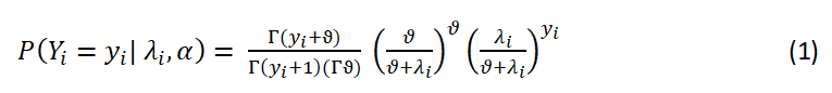
Where λ_i= t_i λ and the dispersion parameter α= ϑ⁻¹

The parameter λ represents the mean incidence rate of response variable y, and it can be used to illustrate the possibility of a repeat of the incident during a specific exposure period t. The mean is

NB regressions transform to Poisson regression in the limit as α→0, and indicate overdispersion when α>0. The negative binomial regression model is expressed as the following form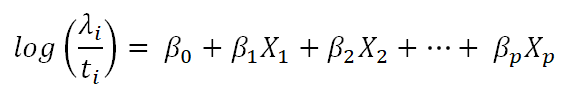

The regression coefficients β₀,β₁,…,β_p are unknown parameters of a set of p repressors that are estimated from a set of data.

Generalized poison regression

The Poisson model is good for modeling discrete counts of events that happen in a fixed space or time interval. The Poisson model is especially useful in situations where counts are right-skewed and thus cannot be reasonably approximated by a normal model. The generalized poison model is appropriate when the observation is over-dispersed [10,11]. The pmf of GP distribution can be defined as:

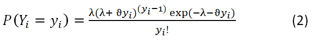
Where, Y_i=0,1,2,… is the random variable, y is count; ϑ is dispersion parameter, 0 ≤ ϑ<1; λ is the rate parameter, λ>0 [12]. The mean of the GP distribution is λ/(1− ϑ), and variance is λ/(1− ϑ)². When ϑ=0 the GP distribution is reduced to the standard Poisson distribution with mean λ. GP regression reduces to Poisson regression when ϑ=0, indicate over dispersion when ϑ>0 (α>0) and under dispersion when ϑ<0 (α<0) [13]. The log-likelihood function (LF) of GP regression is given by [14]:

Where μ_i= (1−ϑ) exp (x_iβ) and λ (μ) is the solution of the preceding equation for the mean. The maximum likelihood estimates can be obtained by maximizing the log-likelihood. Established a generalized poisson distribution that is more flexible in modeling over dispersion than the Poisson distribution. However, it does not belong to the exponential family, sometimes making analysis more difficult.

Conway Maxwell poison regression

The Conway-Maxwell-Poisson distribution is a two-parameter extension of the Poisson distribution that generalizes the Poisson, binomial, and negative binomial discrete distributions, introduced by Conway and Maxwell [15] in the context of queuing systems. It’s useful statistical and probabilistic properties are elegantly derived [16,17]. Its probability function can be defined as.

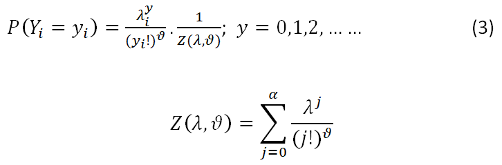
For λ>0 and ϑ ≥ 0. The addition of the scale parameter ϑ enables the ratio (P(Z=j-1))/(P(Z=j))to increase either sub or super-linearly and allows Z to have a variance that is either less than or larger than its mean 16 (the mean of Z ~ CMP (λ, ϑ). With parameter nλ, the CMP approaches an ordinary Poisson distribution, as ϑ=1 (thus Z (λ, ϑ)=exp (λ)). Less than one value of ϑ corresponds to successive ratios that are flatter than the Poisson distribution, hence too long tails or over dispersion.

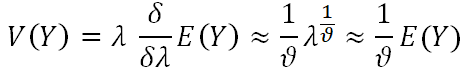
The mean is used to parameterize the Conway-Maxwell-Poisson distribution (family=compois) [18]. To estimate the parameter of CMP 7 showed three methods including the maximum likelihood estimator using iteration (more computationally intensive) and the Bayesian method using conjugate prior, the posterior density of the parameters. For ϑ ≤ 1 or λ>10^ϑ, the mean value and variance of CMP distribution are

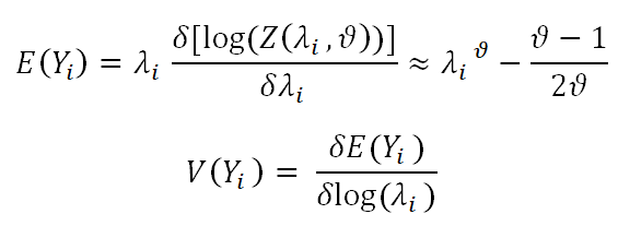
It is worth noting that the useful result for this distribution is E (Y^ϑ)=λ. The relationship between these two moments can be rewritten as

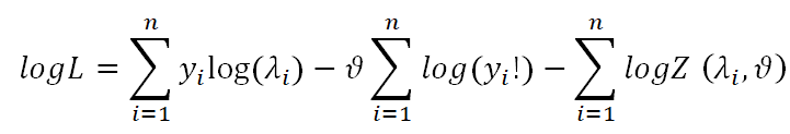
For n independent and identically distributed observations y₁y₂,…, y_n the log-likelihood is given by

CMP is a versatile distribution that can account for overdispersion and underdispersion, both of which are common in count data. It is also easy to use, flexible and performs well in many settings. The advantages with useful several applications (such as in marketing, online auctions, etc.) of using the COM-Poisson distribution are illustrated [19,20].

Case study: COVID-19 death data

Information on COVID-19 cases is taken from the daily reports of the Institute of Epidemiology Disease Control and Research (IEDCR), Dhaka, Bangladesh, from March 8, 2020, to April 30, 2022. Data are accessed from the website. The daily temperature (measured in °C) and humidity (%) of Bangladesh are collected from the link.

Testing for variable dispersion

Sellers and Shmueli developed a hypothesis testing approach to detect whether there is considerable data dispersion, demonstrating the importance of a COM-Poisson regression model over a standard poisson regression model. It can be performed by Likelihood Ratio Test (LRT), H₀: ϑ=0 vs. H₁: ϑ≠ 0. The critical value of the chi-square distribution with a significance level of 2α is used to examine the null hypothesis at the α level of significance. When the LRT value is greater than the chi-square critical value, the null hypothesis is rejected.

LRT=2(lnL₁−lnL₀).

Where lnL₁ and lnL₀ are the models’ log-likelihood under their respective hypotheses.

Akaike Information Criteria (AIC)

When comparing the performance of different models, one can use a variety of likelihood metrics that have been put forth in the statistical literature. AIC is one of the most widely used metrics. A model with more parameters was penalized by the AIC, which is defined as

AIC=2K-2lnL

Where K is the number of independent variables used and L is the log-likelihood estimate. A low AIC value is advantageous for the fitted model.

Results and Discussion

Numerical illustration

Descriptive analysis: As of 8 March 2022 to 30 April 2022, a total of 27514 cases of deaths were officially reported in Bangladesh. This data indicates a positive link between mortality and the daily peak temperatures (person’s r=0.228) and humidity (person’s r=0.295). Table 1 summarizes the descriptive statistics of the number of COVID-19 deaths and the climatic parameters for 764 days. We used a histogram of the observed count frequencies to get a preliminary understanding of the dependent variable.

Table 1. Descriptive statistics of number of daily COVID-19 death and meteorological factors (temperature and humidity).

While the humidity and temperature on average are 30.30°C and 63.67%, respectively, the average daily confirmed death rate from COVID-19 is about 36. The maximum temperature recorded during this pandemic time was 37°C, while the minimum temperature was 21% whereas the highest humidity recorded was 100%.

The number of deaths brought on by COVID-19 is represented by a histogram and a kernel density plot in Figure 1. It indicates that one of the best probability models for this variable is the bell-shaped distribution since it shows that the number of deaths caused by COVID-19 appears to be distributed symmetrically. Although it shows that the total number of deaths linked to COVID-19 has a distributional form that approaches a skewed pattern, it implies that an uneven distribution would be better suitable for predicting the values of this variable.

Figure 2 depicts the scatter plot of the daily number of COVID-19 related deaths against daily temperature, humidity, and time for the time period from March 8, 2020, to April 30, 2022. The response variable and the explanatory variables have an obvious non-linear relationship. These graphs also illustrate a relationship between the experimental variable and covariates.

Regression model fitting and selection: With Poisson, Conway-Maxwell-Poisson, and negative binomial distributions on the conditional model, we fitted GLMMs to the COVID-19 death data and chose the best model. The Conway-Maxwell-Poisson GLMM, which enabled counts to fluctuate with temperature and humidity, was the most cost-effective model we looked at. We offer the summary from more complex models in Table 2 to illustrate the additional output from dispersion models.

Table 2. Summary value for poisson, NB, GP and CMP regression models in glmm TMB for over-dispersed counts of COVID-19 death data in Bangladesh.

The interpretation of coefficients is clearer for the CMP model. After dividing the COM-Poisson coefficients by ν dispersion parameter (0.025/3.53 × 10⁹=7.0821), the results in Table 2 point out that the regression parameters for all models have almost similar estimates in terms of the coefficient magnitudes. The estimated dispersion parameter for COM-Poisson model is ϑ=3.53 × 10⁹, indicating severe over-dispersion, so we can use the approximation

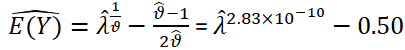
Where is given by: =-0.654+0.080 × temperature+0.025 × humidity

A hypothesis test developed by Sellers and Shmueli is used to determine if the dispersion parameter is significant or not 17 are used. Since the p value is nearly zero, dispersion is present, necessitating a CMP regression as opposed to a poisson regression. Model comparison using information criteria: We may compare all GLMMs, using AIC values. The AIC calculates the model’s relative information value based on the highest likelihood estimate and the number of parameters (independent variables) in the model. We output the table for the working models here. The most parsimonious model feature is the Conway-Maxwell-Poisson distribution with temperature and humidity influences. From Table 3, it is obvious that CMP better fits the model having the smaller AIC value. AIC score variance between the CMP model and the other models under comparison. The third-best model in this Table 3 has a delta-AIC of 197.91 compared to the top model, while the next-best model has a delta-AIC of 100.46 compared to the top model. Additionally, in this instance, 100% of the entire AICc weight is included in the cumulative weight of the top two models.

Table 3. Model selection based on AICc.

Conclusion

The use of discrete distributions to fit discrete data is rare in practice. The Poisson distribution is the most popular, and the negative binomial distribution is frequently employed with over dispersed data. Variations are created when none of the existing distributions seem acceptable. In this way, the Conway Maxwell Poisson (CMP) distribution broadens the selection of discrete distributions available for data modeling. The response variable of interest in this study is a count, meaning it accepts non-negative integer values. The most used regression model for count data is poisson regression. The equidispersion assumption limits poisson regression. The employment of heneralized Poisson and negative binomial regression is a typical solution when data exhibit over-dispersion. In recent years, CMP regression has been utilized to fit distributed data. Generalized Poisson, NB, and CMP regression models are fitted, respectively, to estimate the impact of temperature and humidity on the number of daily deaths. The findings showed that all models’ regression parameters had similar estimates, and generalized and NB models had lesser ratios than Poisson models. Both over dispersion tests showed that NB and COM-Poisson regression were superior to the Poisson model in terms of accuracy. The COM-Poisson has the best-matching terms of log-likelihood and AIC. Based on the results it is obvious that CMP regression provides more accurate results which support its superiority in this context with statistical evidence. Although it is remarkable that a long-forgotten distribution has been revived, we believe that our analysis of its statistical use sheds light on the beauty and use of the CMP distribution. We use a modern method that combines theory and numerical methods to investigate the CMP distribution and other discrete distributions. Only because of today’s more advanced computer power was this made possible.

Author Contributions

Nazmin Akter: Conceptualization; data curation; formal analysis; investigation; methodology; software; visualization; writing-original draft, review and editing. Md. Rezaul Karim: Methodology; supervision; validation; writing-review.

Conflict of Interest Statement

The authors declare no conflict of interest.

Ethics Statement

We have conducted ourselves with integrity, fidelity, and honesty. We have not intentionally engaged in or participated in malicious harm to another person or animal.

Funding

This research received no specific grant from any funding agency in the public, commercial, or not-for-profit sectors. Consent to participate-not applicable, Consent for publication-not applicable.

Availability of Data and Materials

The data are available on the website, and the link is provided in Section 2. It will be provided if anyone requires this. Code availability: The R codes are available. It will be provided if anyone requires this.

References

1. Hilbe, Joseph M. Modeling count data. Cambridge University Press, 2014.

   [Google Scholar]

2. O'Hara, Robert, and Johan Kotze. "Do not log-transform count data." Nat Preced 1 (2010): 1-11.

   [Crossref] [Google Scholar]

3. Rodriguez, German. "Models for count data with overdispersion." Addendum to the WWS 509 (2013).
4. Coxe, Stefany, Stephen G West, and Leona S Aiken. "The analysis of count data: A gentle introduction to Poisson regression and its alternatives." J Pers Assess 91 (2009): 121-136.

   [Crossref] [Google Scholar] [PubMed]

5. Barriga, Gladys DC, and Francisco Louzada. "The zero-inflated Conway-Maxwell-Poisson distribution: Bayesian inference, regression modeling and influence diagnostic." Stat Methodol 21 (2014): 23-34.

   [Crossref] [Google Scholar]

6. Lynch, Heather J, James T Thorson, and Andrew Olaf Shelton. "Dealing with under-and over-dispersed count data in life history, spatial, and community ecology." Ecology 95 (2014): 3173-3180.

   [Google Scholar]

7. Shmueli, Galit, Thomas P Minka, Joseph B Kadane, and Sharad Borle, et al. "A useful distribution for fitting discrete data: revival of the Conway-Maxwell-Poisson distribution." J R Stat Soc C Appl Stat 54 (2005): 127-142.

   [Crossref] [Google Scholar]

8. Karim, Rezaul, and Nazmin Akter. "Effects of climate variables on the COVID-19 mortality in Bangladesh." Theor Appl Climatol 150 (2022): 1463-1475.

   [Crossref] [Google Scholar] [PubMed]

9. Brooks, Mollie E, Kasper Kristensen, Koen J Van Benthem, and Arni Magnusson, et al. "GlmmTMB balances speed and flexibility among packages for zero-inflated generalized linear mixed modeling." RJ 9 (2017): 378-400.

   [Crossref] [Google Scholar]

10. Wang, Guiming. "Bayesian regression models for ecological count data in PyMC3." Ecol Inform 63 (2021): 101301.

    [Crossref] [Google Scholar]

11. Scollnik, David PM. "A Damaged Generalised Poisson Model and its Application to Reported and Unreported Accident Counts." ASTIN Bull J IAA 36 (2006): 463-487.

    [Google Scholar]

12. Consul, Prem C. "Generalized Poisson distributions: Properties and applications." (1989).
13. Ismail, Noriszura, and Hossein Zamani. "Estimation of claim count data using negative binomial, generalized Poisson, zero-inflated negative binomial and zero-inflated generalized Poisson regression models." CAS E-Forum 41 (2013): 1-28.
14. Harris, Tammy, Zhao Yang, and James W Hardin. "Modeling underdispersed count data with generalized Poisson regression." Stata J 12 (2012): 736-747.

    [Crossref] [Google Scholar]

15. Conway, RICHARDSV "A queueing model with state dependent service rate." J Ind Eng 12 (1961): 132.
16. Daly, Fraser, and Robert E. Gaunt. "The Conway-Maxwell-Poisson distribution: distributional theory and approximation." Latin Ame J Probabil Mathematic Statis 13 (2016): 635-658.

    [Crossref] [Google Scholar]

17. Sellers, Kimberly F, and Galit Shmueli. "A flexible regression model for count data." Ann Appl Stat 4 (2010): 943-961.

    [Google Scholar]

18. Huang, Alan. "Mean-parametrized Conway-Maxwell-Poisson regression models for dispersed counts." Stat Model 17 (2017): 359-380.

    [Crossref] [Google Scholar]

19. Borle, Sharad, Peter Boatwright, and Joseph B Kadane. "The timing of bid placement and extent of multiple bidding: An empirical investigation using eBay online auctions." Statist Sci 21 (2006): 194-205.

    [Google Scholar]

20. Borle, Sharad, Peter Boatwright, Joseph B Kadane, and Joseph C Nunes, et al. "The effect of product assortment changes on customer retention." Mark Sci 24 (2005): 616-622.

    [Crossref] [Google Scholar]