Assessment of the Climatic and Environmental Factors on the Spatial Distribution of Malaria in Amhara Region, North-West Ethiopia

Haile Mekonnen Fenta¹, Lijalem Melie Tesfaw¹, Awoke Seyoum Tegegne¹, Denekew Bitew Belay¹, Godada Keleb Lake¹, Muluwork Ayele Derebe¹, Abay Kassa Teklie^1*, Eyerus Asmare¹ and Mollalign Tarekegn Minwagaw^2
*Correspondence: Abay Kassa Teklie, Department of Statistics, College of Science, Bahir Dar University, Bahir Dar, Ethiopia, Email:

Keywords

Malaria prevalence • Malaria incidence • Amhara region • Spatio-temporal distribution • Moran’s I index

Abbreviations

GNS: General Nesting Spatial; SAC: Spatial Autocorrelation; SDM: Spatial Durbin Model; SDEM: Spatial Durbin Error Model; SAR: Spatial Autoregressive; SLX: Spatial Lag of X; SEM: Spatial Error Model; OLS: Ordinary Least Squares; DLST: Daytime Land Surface Temperature; EVI: Enhancement of Vegetation Index; NLST: Nighttime Land Surface Temperature; DTR: Diurnal Temperature Range; ITN: Insecticide-Treated Bed Nets; LST: Land Surface Temperature

Introduction

Malaria is an acute febrile illness and life-threatening disease caused by parasites called Plasmodium parasites that are transmitted to people through the bites of infected female Anopheles mosquitoes. Although there are many species, there are mainly 5 parasite species that cause malaria in humans, and 2 of these species–P. falciparum and P. vivax–pose the greatest threat. P. falciparum is the deadliest malaria parasite and the most prevalent on the African continent [1]. Since 2000, malaria case incidence had reduced from 368 to 222 cases per 1000 population at risk in 2019, before increasing to 233 in 2020 owing to disruptions during the COVID-19 pandemic. Between 2000 and 2019, malaria deaths reduced by 36%, from 840,000 in 2000 to 534,000 in 2019, before increasing [2]. There were 241 million cases of malaria in 2020 compared to 227 million cases the previous year which is 2019 and the estimated numbers of malaria deaths were 627,000 in 2020 and 558,000 in 2019. The WHO African region carries a disproportionately high share of the global malaria burden. In 2020, the region was home to 95% of malaria cases and 96% of malaria deaths. Children under 5 accounted for about 80% of all malaria deaths in the region [2,3].

According to a WHO report, there was a decline in both new cases and the mortality rate of malaria. But both the incidence and mortality rates showed an increase in mortality rate and incidences of malaria [1]. The WHO African region carries a disproportionately high share of the global malaria burden. In 2020, the region was home to 95% of malaria cases and 96% of malaria deaths. Children under 5 accounted for about 80% of all malaria deaths in the region.

Malaria has an estimated incidence of more than 300 million new cases every year worldwide. About one million people die each year due to malaria, of which most of them are in sub-Saharan Africa [1-4]. Approximately 90% of malaria cases are related to environmental factors [5]. In Ethiopia three-fourths of the land below 2000 meters of altitude is malarious, in which two-thirds of the country’s population is at risk of malaria infection. In Ethiopia alone there is an average of 5 million cases a year, causing 70,000 deaths each year and accounting for 17% of outpatient visits to health institutions [6]. It has been argued that economic growth is dependent on two key factors. The main objective of the current investigation was to assess the climatic and other environmental predictors for the spatial distribution of malaria in the Amhara region, Northwest Ethiopia.

Materials and Methods

Study area

The study is conducted in Amhara regional state, the second populous among 11 Ethiopia’s regional states. The region covers almost 16% of the country areas and it is composed of 11 administrative zones and 109 woredas. It is bound by the states of Benishangul/Gumuz in the Southwest, Oromia in the South, Afar in the East, Tigray in the North, and the Republic of Sudan in the West. For further information, refer to Figure 1.

Figure 1. Geographical location of Amhara region with reference to the national map of Ethiopia.

The region’s annual rainfall ranges roughly from 770 mm in the lowlands to 2000 mm in the highlands. Seasonal variations of temperature range from 16°C in the wet season to 27°C in the dry season. Cropland and pasture are the two main forms of land cover in the area, and rain-fed agriculture is the primary source of agricultural production [7]. The region's malaria transmission is unstable [8]. The main epidemic season of malaria in the region is from September to December following the summer rainy season from June to August [9].

The data

For this analysis, we used two sources of data sets. The first source is from Amhara Public Health Institute (API) records. The second data set is from the Ethiopian demographic and health survey of 2000, 2005, 2011, and 2016 which is used to obtain the geospatial covariates. The EDHS has GPS coordinates associated with covariate datasets (in both raster and vector Geographic Information System (GIS) formats) to facilitate spatial analysis which links survey cluster locations to ancillary data called covariates [10] that contain data on climate, population, and environmental, and other factors.

In this manuscript, the independent variables were extracted from Ethiopian Demographic and Health Survey and joined with malaria incidence (cases per 1000 people per year) with proximity to ware (km), vegetation (0~1), rainfall, and population distribution (population per hectare) data for DHS clusters (Enumeration Areas: EA). The EDHS geospatial covariates of survey cluster locations in Ethiopia to environmental, demographic, and climate data covariates allow for more advanced spatial analysis of malaria (Table 1).

Table 1. Climate and environmental covariates, and their definitions from EDHS.

Methods

The traditional linear regression models estimated by the ordinary least squares methods cannot take into account the fact that data collected based on spatial specifications is not independent of its spatial location [11]. Hence the observed values cannot remain independent because the closeness of the locations may cause relevance; and if the spatial effect is neglected in the model, the estimation values will be biased [12,13]. As a result, spatial weight (W) is introduced for adjusting the relationships between dependent variables and, independent variables, and the residual terms to reflect the spatial interaction relations with the dependent variables.

The unit of the prevalence of malaria was measured in terms of percentage, which is the ratio of total positive and total tests multiplied by 100. For the convenience of computations, the 93 different woredas were represented using identification numbers 1, . . . ,93. The number of positive malaria cases observed in the woreda i (i=1, 2, . . ., 93), denoted by yi, was assumed to follow a Poisson distribution with mean λi=Eiγi, where Ei (offset term, which is used as a correction factor for the model) [14,15] denotes the number of expected cases (malaria cases) in woreda i, and γi is the relative risk for woreda i. Moreover, Ei was calculated as

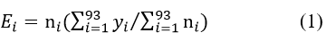
where n_i is the number of tested cases in woreda i [16-18]. The spatial matrix can be constructed in many ways depending on the definition of the neighborhood employed (Figure 2). The simplest way is to construct a binary connectivity matrix [19,20].

Figure 2. Different spatial weight matrices.

The two areas are neighbors if they are spatially contiguous.

The elements of w_ij are (i, j), which is the neighborhood structure between the observations as n × n matrix W in which the elements w_ij of the matrix are the spatial weights:

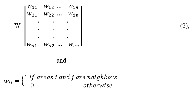
The size of the matrix is equal to the number of zones. The existence of spatial autocorrelation and the proper weight matrix (W) in the dataset is checked by using Moran’s I. Moran’s I am used to associate weight (W_ij) to each of the pairs, which quantifies the spatial pattern. The test is given as follows:

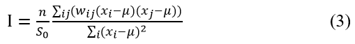
where n: number of investigated points; x_i, x_j: the observed value of two points of interest; μ: the expected value of x; wij: the elements of the spatial weight matrix; and S₀: normalize S₀=Σ_ijw_i,j. The Moran’s I ranges [-1, 1], of which the value of 1 signifies that clusters with high malaria cases are close to clusters with similar high cases, while -1 indicates that high values are near to low values. After confirming the presence of spatial autocorrelation across the study areas, it might be due to the fact that the correlation in the distribution of malaria cases leads to the correlation among the error terms, thereby rendering the Ordinary Least Square (OLS) estimator inappropriate owing to the violation of the assumptions [11].

Hence, the seven models were proposed. The three different types of interactions in the listed spatial model have been divided into the outcome interaction effects between the explained variable (Y), the covariates interaction effects between the explanatory variables (X), and the interaction effects between the error terms (ε).

Let ρ be the spatial lag parameter, λ be the spatial autoregressive parameter, W be the spatial weight matrix, X be the explanatory vector of variables, β be the corresponding parameters vector, and ε be the error term which is identically and independently distributed. The variable in the model WY denotes the spatial interaction effects among the dependent variables, WX is the interaction effects among the covariates and the Wu is the interaction effects among the error terms of different observations. The performance of the given models was compared by using Akaike’s and Bayesian Information Criteria (BIC). The spatial effects model is summarized in Figure 3.

Figure 3. Different spatial models.

Results

Data visualization was done using numerous summary statistics for each covariate and spatial plots for the prevalence of malaria in the Amhara region. Table 2 revealed some common summary statistics such as minimum, maximum, first quartile, median, third quartile, mean, and standard deviation computed from each covariate considered in this study. The minimum and maximum precipitation were 45.30 and 115.58 mm respectively. A quarter of woredas in the Amhara region had precipitation equal to 73.67 mm.

Table 2. Summary statistics of the covariates considered in the study.

The line graph for the prevalence of malaria across districts (descending order) for the last five years (2016-2022) is indicated in Figure 4. It revealed that the highest prevalence of malaria in the three successive years (2016-2018) was obtained in the Beyeda district, whereas, for the last two consecutive years (2019-2020), Asagirt and Gozamin districts were ranked first and second most malaria prevalent districts respectively. For instance, among the total population who were tested in the Asagirt Hospital, 83.3% of the people who were malaria tested positive. In contrast, the lowest malaria occurrence in 2016 and 2017 was obtained in Bahir Dar city. Moreover, Kombolcha town, Gishe and Kutaber districts had the lowest occurrence of malaria in 2018, 2019, and 2020 respectively. On average, about 18% (with a standard deviation of 13%) of individuals who visited the hospitals for checkups became malaria positive. The minimum prevalence of malaria, in the study area, was 1.89% and the maximum prevalence was 83.3%.

Figure 4. Line plot of malaria prevalence across districts in 2016- 2020.

The prevalence of malaria among the administrative woredas in the Amhara region of Ethiopia is indicated in Figure 5. Prior to computing the prevalence of malaria, total tests and total positives were identified. The special prevalence of malaria for each woreda was also evaluated for five successive survey years (2016-2020) as shown in Figure 5. Despite some improvement noticed from the year 2016 to 2020, it can be seen that a considerable prevalence of malaria has occurred in the region.

Figure 5. The special prevalence of malaria among different woreda in the Amhara region, Ethiopia.

The spatial autocorrelation report of malaria among woredas was conducted using Moran’s I statistics as indicated in Figure 6. The Moran’s I index statistic was 0.217758 with a corresponding P-value of 0.014139 which is less than 0.05 and this indicates that the spatial autocorrelation of malaria across woredas was statistically significant. The positive Moran’s I statistic indicates a woreda with a higher prevalence of malaria surrounded by a woreda that has a higher prevalence of malaria and vice versa.

Figure 6. Moran’s I index plot of spatial autocorrelation report.

For a better and easier understanding of policymakers, planners, and other stakeholders who are interested to read this paper about malaria prevalence in the Amhara region, a hot spot analysis was conducted as shown in Figure 7. The woreda with red highlighted color indicates there is a hot spot or high prevalence of malaria and in contrast woredas with blue color refers to a cold spot or low prevalence of malaria. Overall, in Figure 7 it can be seen that except in some parts of eastern Amhara, a high prevalence of malaria was noticed across woredas.

Figure 7. Hot spot analysis of malaria across woredas in the Amhara region.

The estimated effects of each characteristic obtained from woredas were computed using OLS and spatial models (SLX, SDM, SAR/SLM, SDEM, SEM, SAC, and GNNS) to explain the prevalence of malaria as indicated in Table 3. Once the effect of each characteristic was estimated using these models, the best model was also identified using AIC, considering a model with a small AIC that better fits the data. Thus, the SAC approach with an AIC value equal to -136.73 is best as compared to other approaches.

In Table 3, it is indicated that the variables Aridity, DSLT, DTR, Temperature, EVI, ITN, LST, N composite, NLST, Water, and wet day of the woredas had a significant effect on the prevalence of malaria. Aridity, DLST, Temperature, EVI, N composite, and NLST had statistically negative effects while DTR, ITN, LST, water, and the wet day had a statistically positive effect on the prevalence of malaria.

Table 3. Parameter estimates of OLS and spatial models to explain the prevalence of malaria.

Table 3 indicates that Aridity had a negative association with the prevalence of malaria in the study area. Hence, as aridity or drought increased by one unit, the expected prevalence of malaria was decreased by 0.019 given the other covariates constant (pvalue< 0.001). Temperature also significantly affected the prevalence of malaria in the study area. Hence, as temperature increased by onedegree centigrade, the corresponding prevalence of malaria was decreased by 0.438, given the other covariates constant (pvalue< 0.01). Similarly, as the enhancement of vegetation increased by one unit, the expected prevalence of malaria was decreased by 0.001 given the other covariates constant (p-value<0.001). Land Surface Temperature (LST) had a significant effect on the prevalence of malaria in this study. Hence, as LST increased by one unit, the expected prevalence of malaria also increased by 11,436, given all other covariates constant (p-value<0.001).

The average number of days receiving rainfall within the 2 km for urban or 10 km for rural buffer surroundings also statistically and significantly affected the prevalence of malaria. This was named a wet day. Hence, as the wetness of the day increased by one unit, the expected prevalence of malaria also increased by 0.037, assuming that all other covariates remain constant (P-value<0.05).

Daytime Land Surface Temperature (DLST) had a significant effect on the prevalence of malaria in the study area. Table 3 indicates that as DLST increased by one unit, the expected prevalence of malaria decreased by 5718, given the other covariates constant (pvalue< 0.001). Similarly, Diurnal Temperature Range (DTR) had a statistically significant effect on the variable of interest. Hence, as DTR increased by one unit, the expected prevalence of malaria was 0.1082, given that the other covariate remains constant (pvalue< 0.001).

As the proportion of the population protected by Insecticide- Treated Bed Nets (ITN coverage) increased by one unit, the expected prevalence of malaria was also increased by 0.001 (p-value<0.01) given that the other conditions remained constant. Similarly, as the amount of water (Stagnant water) increased by one unit, the expected prevalence of malaria was also increased by 0.001, assuming all other covariates were constant (P-value <0.05).

The average nighttime luminosity (N-composite) significantly affected the prevalence or distribution of malaria in the study area. Hence, as the N-composite increased by one unit, the expected prevalence of malaria was decreased by 0.015, given the other covariates constant (p-value<0.01).

Discussion

In drought areas the prevalence of malaria is weak; the potential reason for this may be the low survival rate of Anopheles mosquitoes for implementation of its regular activities. This result is supported by one of the previous studies. Hence, Anopheles mosquitoes might get difficulty conducting its day-to-day activities. The result of the previous study states that malaria transmission in arid and semi-arid regions is often influenced by climatic factors. The relationship between climate variables and malaria transmission dynamics is therefore instrumental in developing effective malaria control strategies.

The prevalence of malaria is very low in very high temperatures or very cold temperature areas. It is known that in a drought area, the temperature is very high, which is difficult for the survival of Anopheles mosquitoes. Hence, the very cold and very hot temperatures can have difficult situations for the distribution of malaria, because of the nonfavorable conditions for the vector Anopheles mosquito. This result is also supported by one previously conducted research. One of the previous studies stated that the spatial variations of malaria in TE18 and TE15 indicate a very practical limitation of using elevation alone to demarcate regions with or without epidemic malaria. The role of temperature in malarial epidemics was demonstrated by a retrospective study of malarial cases in the highland region of East Africa from 1970 to 2003. This study found an association between malaria epidemics and warmer temperatures. Hence, warm temperature favors the survival of malaria-carrying mosquitoes, but the degree to which a rise in temperature increases the spread of malaria is dependent on the baseline temperature, with cooler regions experiencing the largest change.

Previously conducted research has shown that there is a nonlinear relationship between the Extrinsic Incubation Period (EIP) and temperature. EIP is very temperature sensitive in that small changes in the latter may result in significantly large effects on malaria transmission. Thus, as temperature increases, mosquitoes become infectious quickly due to a shortened EIP and vice versa. Hence, the, respectively, negative and positive association of minimum and maximum temperatures with malaria incidence is somewhat suggestive of the nonlinear relationship between the two variables (i.e., temperature and malaria) as mentioned earlier.

The enhancement of the vegetation index has a negative effect on the distribution of malaria. Densely populated vegetation leads to the reduction of the prevalence of malaria. This result is consistent with one of the previous studies which stated as a reduction of malaria risk occurred when there is moderate vegetation cover compared to sparse vegetation cover. Another investigation states that local vegetation cover is a risk factor for malaria transmission.

Land Surface Temperature (LST) can affect the prevalence of malaria. It is known that a humid land surface has a high prevalence of malaria which is known as a malarious area. The potential reason for this might be the fact that humidity is a favorable condition for the survival of Anopheles mosquitoes as compared to drought areas. This result is in line with another previously conducted research. Hence, Land Surface Temperature (LST) is used as a proxy for monitoring minimum air temperature which is one of the factors of mosquito development time as well as an indicator of Plasmodium parasite development within the mosquito vectors. A minimum air temperature of ≥ 18°C is a necessary condition for potential Plasmodium falciparum malaria prevalence while a minimum temperature of ≥ 16° C is considered a necessary condition for Plasmodium vivax transmission.

Daytime Land Surface Temperature (DLST) was one of the variables having a significant effect on the variable of interest. Hence, a very high DLST value leads to a decrease in the prevalence of malaria. In many studies regarding the field of malaria, time factors have been acquired in single-time, multi-time, or short-time series using remote sensing and meteorological data. Selecting the best periods of the year to monitor the habitats of Anopheles larvae can be effective in better and faster control of malaria outbreaks.

The higher the value of wetness of the day leads to the favorable condition for the survival of Anopheles mosquito and this further leads to the high prevalence of malaria. Rainfall had a positive correlation with malaria occurrences. This indicates the increased risk of malaria transmission during rainy times. Similar findings were also reported from different areas of the country and elsewhere in the world. A study in Southwest Ethiopia also reported that mean rainfall has a positive correlation with malaria incidence.

The high fluctuation of temperature within a given day leads to the high prevalence of malaria in the study area. The result of the previous study indicates that high-risk times (high-temperature range) are associated with an increase in the abundance of Anopheles mosquitoes. As such, climate change is most likely to increase the spread of malaria associated with the breeding of the mosquito vector.

Areas with high amounts of water (Stagnant water) are favorable conditions for the breeding of Anopheles mosquitoes and this further leads to the high prevalence of malaria. The result of the previous study states that malaria parasite infection was linked to a history of malaria and the presence of stagnant water near a home.

The average nighttime luminosity (N-composite) significantly affected the prevalence or distribution of malaria in the study area. Hence, the higher average nighttime luminosity is associated with a decrease in the prevalence of malaria. This result is in line with the result obtained in one of the previous studies. It is known that the average nighttime luminosity in urban areas is better as compared in rural areas. The result obtained in one of the previous studies indicates that the higher urban city is significantly associated with a lower household density of mosquitoes.

Conclusion

The prevalence of malaria across Amhara districts was considerably high and a remarkable positive spatial autocorrelation of the prevalence of malaria across districts was observed. The highest prevalence of malaria was observed in Asagirt Woreda. Among the covariates, aridity, temperature, the enhancement of vegetation, land surface temperature, daytime land surface temperature, daytime wet, and range of temperature variation, amount of rainfall/stagnant water, and average nighttime luminosity statistically affected the prevalence of malaria in the study area. Among these, aridity, DLST, temperature, EVI, N-composite, and NLST had statistically negative effects while DTR, ITN, LST, water, and the wet day had statistically positive effects on the prevalence of malaria.

As a recommendation, health-related education should be strengthened on removing stagnant water by discarding old tires that may collect rainwater, and removing debris from streams so streams flow more freely. The Amhara public health institute including the health Bureau, stakeholders, and all concerned bodies should give special attention should be given to the highest malaria districts of the West Gondar zone.

Limitation of the Study

Though the data considered in this study are more than enough to represent the region, it can be considered as a limitation that in some of the woredas the prevalence of malaria was not accessible.

Ethical Approval and Consent to Participate

All methods were carried out in accordance with relevant guidelines and regulations. This was approved by the Bahir Dar licensing committee, in Ethiopia.

Consent for Publication

This manuscript has not been published elsewhere and is not under consideration by any other journal. The authors agreed this manuscript be submitted to this journal for publication.

Availability Data and Privacy Regulations

The data used in the current investigation is available to the corresponding authors. The data accessed in the current investigation complied with relevant data protection and privacy regulations, and this study was conducted in accordance with the Declaration of Helsinki.

Authors Contribution

AS proposed the plan. HMF, LMT, DBB, and AST arranged the data and wrote the manuscript. MA, GK, MT, and AK edit and revise the manuscript. Finally, all authors edit and approved the manuscript.

Funding

Not applicable

Disclosures

The author declared that there is no conflict of interest regarding the publication of this manuscript.

References

1. Chenciner, Louisa, Kristi Sidney Annerstedt, Julia M. Pescarini, and Tom Wingfield. "Social and health factors associated with unfavourable treatment outcome in adolescents and young adults with tuberculosis in Brazil: a national retrospective cohort study." Lancet Glob Health 9 (2021): e1380-e1390.

   [Crossref] [Google Scholar] [PubMed]

2. Yovo, Emmanuel. "Challenges on the road to achieving the SDG 3.2 targets in resource-limited settings." Lancet Glob Health 10 (2022): e157-e158.

   [Crossref] [Google Scholar] [PubMed]

3. Belay, Denekew Bitew, Yehenew Getachew Kifle, Ayele Taye Goshu, and Jon Michael Gran, et al. "Joint Bayesian modeling of time to malaria and mosquito abundance in Ethiopia." BMC Infect Dis 17 (2017): 1-12.

   [Crossref] [Google Scholar] [PubMed]

4. Hawaria, Dawit, Solomon Kibret, Assalif Demissew, and Arega Tsegaye, Denekew Bitew, et al. "Survivorship of Anopheles gambiae sensu lato in irrigated sugarcane plantation scheme in Ethiopia." Parasit Vectors 14 (2021): 1-10.

   [Crossref] [Google Scholar] [PubMed]

5. Zemene, Endalew, Denekew Bitew Belay, Abebaw Tiruneh, and Ming-Chieh Lee, et al. "Malaria vector dynamics and utilization of insecticide-treated nets in low-transmission setting in Southwest Ethiopia: implications for residual transmission." BMC Infect Dis 21 (2021): 882.

   [Crossref] [Google Scholar] [PubMed]

6. Desta, Lakew. "Land degradation and strategies for sustainable development in the Ethiopian highlands: Amhara Region." Vol. 32. ILRI (aka ILCA and ILRAD) (2000).
7. Graves, Patricia M, Frank O. Richards, Jeremiah Ngondi, and Paul M. Emerson, et al. "Individual, household and environmental risk factors for malaria infection in Amhara, Oromia and SNNP regions of Ethiopia." Trans R Soc Trop Med Hyg 103 (2009): 1211-1220.

   [Crossref] [Google Scholar] [PubMed]

8. Midekisa, Alemayehu, Gabriel Senay, Geoffrey M. Henebry, and Paulos Semuniguse, et al. "Remote sensing-based time series models for malaria early warning in the highlands of Ethiopia." Malar J 11 (2012): 1-10.

   [Crossref] [Google Scholar] [PubMed]

9. Anselin, Luc. "Spatial econometrics: methods and models." Vol. 4. Springer Science and Business Media (2013).
10. Hao, Yu, and Yi-Ming Liu. "The influential factors of urban PM2. 5 concentrations in China: a spatial econometric analysis." J Clean Prod 112 (2016): 1443-1453.

    [Crossref] [Google Scholar]

11. Tobler, Waldo R. "A computer movie simulating urban growth in the Detroit region." Econ Geogr 46 (1970): 234-240.

    [Google Scholar]

12. Blangiardo, Marta, and Michela Cameletti. "Spatial and spatio-temporal Bayesian models with R-INLA." John Wiley and Sons (2015).
13. Haining, Robert, Jane Law, and Daniel Griffith. "Modelling small area counts in the presence of overdispersion and spatial autocorrelation." Comput Stat Data Anal 53 (2009): 2923-2937.

    [Crossref] [Google Scholar]

14. Wang, Feifei, Jian Wang, Alan E. Gelfand, and Fan Li. "Disease mapping with generative models." Amer Statist 73 (2019): 213-223.

    [Crossref] [Google Scholar]

15. Briz-Redón, Álvaro. "The impact of modelling choices on modelling outcomes: a spatio-temporal study of the association between COVID-19 spread and environmental conditions in Catalonia (Spain)." Stoch Environ Res Risk Assess 35 (2021): 1701-1713.

    [Crossref] [Google Scholar] [PubMed]

16. Adeyemi, Rasheed A, Temesgen Zewotir, and Shaun Ramroop. "A Bayesian hierarchical analysis of geographical patterns for child mortality in Nigeria." Open Public Health J 12 (2019).
17. Duncan, Earl W, Nicole M. White, and Kerrie Mengersen. "Spatial smoothing in Bayesian models: a comparison of weights matrix specifications and their impact on inference." Int J Health Geogr 16 (2017): 1-16.

    [Crossref] [Google Scholar] [PubMed]

18. Getis, Arthur, and Jared Aldstadt. "Constructing the spatial weights matrix using a local statistic." Geogr Anal 36 (2004): 90-104.

    [Crossref] [Google Scholar]

19. Fischer, Manfred M, and Jinfeng Wang. "Spatial data analysis: models, methods and techniques." Springer Science and Business Media (2011).

    [Google Scholar]

20. Moran, Patrick AP. "Some theorems on time series: II the significance of the serial correlation coefficient." Biometrika 35 (1948): 255-260.

    [Crossref] [Google Scholar]