Temperature Variation in Transient State of a Thermal Insulator and the Time Fractional Diffusion Equation

Rasolomampiandry G^1*, Rakotoson R² and Randimbindrainibe F^3
*Correspondence: Rasolomampiandry G, Cognitive Sciences and Applications Research Laboratory, BP 1500, Ankatso - Antananarivo 101, Madagascar, Email:

Keywords

Fractional diffusion equation • Experimental results • Thermisorel

Introduction

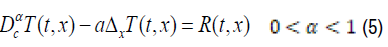
In [1], a heat transfer study was performed on a sample of low density wood fiber board, called Thermisorel. This material is manufactured by STEICO Casteljaloux in France. Thermisorel is used in construction because they avoid heat loss in winter due to their low thermal conductivity, nearly 0.042 W m-1 K-1. It also protects the building from heat in summer due to their capacity high thermal storage.

Details of the study are described in [1]. Only the data necessary for our problem mentioned above, which we will recall.

This work will be divided into three parts:

In section 2, we will perform a discretization of the time fractional diffusion equation. The third part consists in extracting all the data necessary to solve our problem. In particular the experimental results on the on the variation of the temperature, in transient mode, during the heating of this thermal insulator. In the next part, we will develop the fractional diffusion equation according to the data obtained in [1]. Then we will do its numerical resolution, in order to be able to compare the results with the experimental data.In this study we used a 22.2 mm thick thermisorel board

Discretization of the fractional thermal diffusion equation

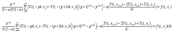
We will only consider the one-dimensional case, i.e. the temperature depends only on the real variable x and the time t. The time fractional thermal diffusion equation is written:

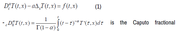
derivative of order α,

where of the real variable t, t>0 [2,3]

- ‘a ’is the diffusivity coefficient

T(t, x) is the temperature corresponding to the variables t and x

f (t, x) is the second member of equation (1) for the variables t and x

For our discretization:

On the segment [0,T₀ ], we construct a finite sequence such that

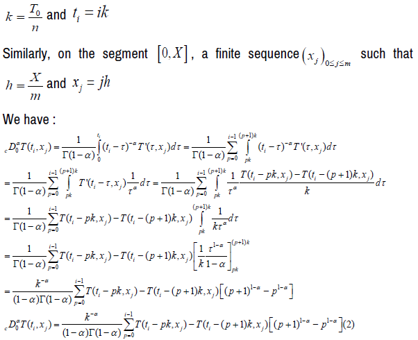
This relation is valid for i ≠ 0

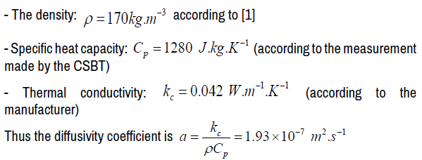
For the discretization of the Laplacian one will use the advanced decentered differentiation [4] and we have:

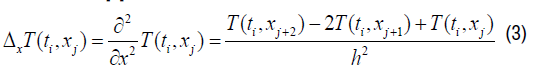
Note:

The equation (1) has become:

Brief Description and Results of the Experiment

Experimentation

As already mentioned above, that in [1], a study on the transient heat transfer on thermal insulation was made. During the experiment, we took a sample of thermisorel plate of thickness E = 22.2mm. The sample was placed between the two plates of a flowmeter and the following temperature specifications were used:

The temperature of one plate should be kept at 15.4 °C and the other plate should raise the temperature from 15.4 to 24.7° C.

The heat flux between the samples and each plate was measured. The same initial temperature was measured (approximately 15.4°C). The temperature rise took several minutes and measurements were taken every 10 second until steady state was reached.

The heat flux measurements were carried out by the CSTB (Scientific and Technical Center for Building) in Grenoble. For the results of this experiment see [1]

The macroscopic properties of the thermisorel

Several properties of this material are mentioned in [1]. In this paragraph, only the parameters necessary for the resolution of our problem we will recall:

Note:

According to [1], the heat transfer by convection and by radiation are negligible, so only the heat transfer by conduction is considered.

Experimental results obtained for the thermisorel

In [1], there are two results of the experiment which are given as a graphical representation. One represents the change in temperature and the other the flux, as a function of time, on both sides of the thermisorel sample.

From these graphs, we extracted the values of the temperature and those of the flux as a function of time, until the steady state was reached, for the hot side. We have the following (Tables 1 and 2)

Numerical resolution of the time fractional thermal diffusion equation

To study the temperature variation on the hot face of the thermisorel, it suffices to study an arbitrary point on this face. From this point, we will consider a straight line segment of length E = 22.2mm and which is perpendicular to the face. On which, we will define a time fractional thermal diffusion equation on segment, including the unknown is the temperature at time t at a point of abscissa x on this line segment, denoted T (t, x).

The equation of the problem

From (1) the equation takes the form:

The radiation effect and the convection effect are negligible, but the existence of the heat source must be considered so we can assume that the corresponding equation is with second member:

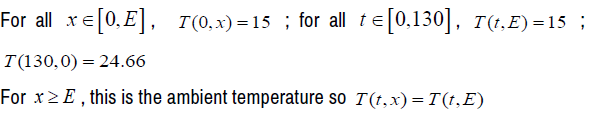
For the initial conditions we have:

The transient regime lasts 130 seconds, then t ∈[0,130]

The length of the line segment is 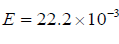meters, then x∈[0, E]

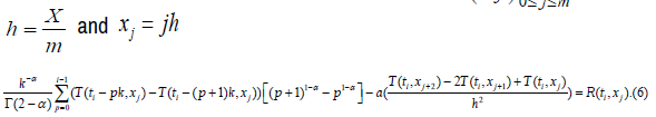
The discretization gives us:

- On the segment [0,130] , we build a finite sequence such that

is equal to the flux observed at the instant on the hot face (see table 2)

- Similarly, on the segment [0,E] , a finite sequence such that

As in the experiment, we will give the values T(t,0) for t ∈[0,130]

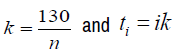
For that ,we will take h = E and k = 10 then 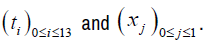And we write (6) by taking j = 0and 0 <i≤13

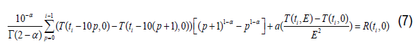
Relation (7) is the discretization corresponding to the time fractional thermal diffusion equation, in accordance with the hypothesis of the experiment.

Numerical resolution

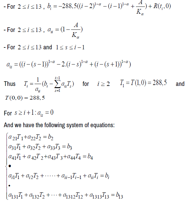
According to the results obtained in the previous paragraph, our problem turns to finding values of This requires a system of 13 equations with 13 unknowns that we will build from (7), as follows:

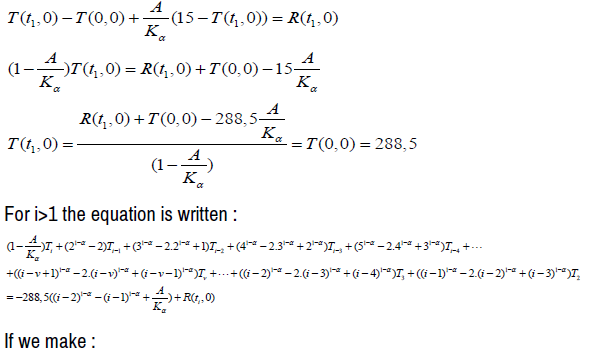
We will write (7) for i = 1,....,13 :

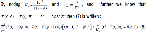
From (8) We obtain a system of Thirteen equations with thirteen unknowns, whose unknowns are as following :

The first equation is:

Numerical resolution and results

With the hypotheses described previously, the method of Gauss and starting from the software MATLAB. We have the graph representing the experimental data and the theoretical results when α = 0.9. And according to the calculation under MATLAB, the difference between the values of the temperature resulting from the experimental method and the values obtained by simulation is 10.09% on average. This percentage is largely sufficient to confirm the adequacy of the experimental data with the theoretical values obtained, from the fractional diffusion equation with respect to time, when α = 0.9 (Figure 1&2).

Conclusion

From these results, we can say once again that we should not be content to use classical derivatives, in the studies of phenomena which require differential equations.

References

1. Kaemmerlen A. Asllanaj F, Sallée H, Baillis D and  Jeandel G. “Transient modeling of combined conduction and radiation in wood fibreinsulation and comparison with experimental data.” Int. J. Therm. Sci. 49(2010): 2169-2176
2. Kilbas Anatoly, Srivatastava Hari M and Trujilio Juan J.  “Theory and applications of fractional differential equations.’’  Elsevier 2006.
3. Podlubny Igor. “ Fractional Differential equations.’’ Elsevier1999.
4. Buffat Pr Marc “ Approximation des dérivées par différences’’
5. Yang Q,  Liu F and Turner I. “ Numericals methods for fractionnal partial differential equations with Riesz space fractionnal derivatives. School of Mathematical Sciences.’’   Appl. Math. Model.34(2010): 200-218.