Research Article - (2022) Volume 11, Issue 11
Received: 02-Nov-2022, Manuscript No. idse-22-77601;
Editor assigned: 03-Nov-2022, Pre QC No. P-77601;
Reviewed: 16-Nov-2022, QC No. Q-77601;
Revised: 17-Nov-2022, Manuscript No. R-77601;
Published:
24-Nov-2022
, DOI: 10.37421/2168-9768.2022.11.355
Citation: Gutu, Abebe Besha. “Optimization of Canal Cross Section for Minimum Seepage Loss: Increasing Net Benefit from Crop Production (Case Study of Korir Irrigation Scheme Kiltie Awlalo Woreda).” Irrigat Drainage Sys Eng 11 (2022): 355.
Copyright: © 2022 Gutu AB. This is an open-access article distributed under the terms of the Creative Commons Attribution License, which permits unrestricted use, distribution, and reproduction in any medium, provided the original author and source are credited.
The objective of the research is minimizing the seepage losses from irrigation canals while increasing the benefit from crop production in Eastern zone of Tigray Region Tabia Genfell, Kilite awulalo woreda korir Irrigation Scheme. During the design of canal the cropping pattern selected were pepper, cabbage, potato, tomato and onion for dry season and maize, wheat, teff, barley and pea for wet season. Realizing that the single crop cannot solve the food security and economic status of the farmers, this research was aimed to solve the problem by using the original cropping pattern along with optimization of canal cross-sections to minimize the shortage of discharge and maximize the net benefit. Accordingly, the linear programming (LP) model formulated, under different scenarios to obtain maximum benefit. The model developed under full design (assumption of no losses), existing condition (under measured seepage), under optimum discharge (minimum seepage) and lastly under optimum discharge and new proposed area and their result were compared to each other in terms of area allocation, maximum profit and saved discharge. The objective function of the model is maximization of net benefit and the constraints of the model were minimum area to be irrigated, maximum area under each secondary canal, constraints of seed and fertilizer cost and constraint of optimum discharge in canals. The result of maximum benefit scenario allocates the minimum required area for pepper, cabbage, potato and onion by allocating 62.5ha, which is maximum area for tomato crop. In terms of saving discharge, the existing condition and scenario IV first condition similar with value of 65% however despite of their saved water, the benefit of existing scenario (scenario II first crop pattern) less by 10% than scenario IV 1st crop pattern. The replacement of cabbage with spinach and potato with carrot in scenario IV second crop pattern save 75% of canal discharge but the net benefit reduced by 2,401,350.00 ETB from scenario IV first condition. In terms of saved discharge during optimization of canal cross-section 20%, 68%, 86%, and 69% amounts of discharge saved from Sc-1, Sc-2, Sc-3 and Sc-4 respectively when compared with existing condition.
Cropping pattern • Optimal • Linear programming • Lagrange multiplier • Seepage • Canal
Background
Agriculture is the main source of the world food production and it covers 70 to 85% of the food supply [1]. Global agricultural production is highly dependent on irrigation; however, efficiencies of irrigation systems are often astonishingly low. Moreover, in arid and semi-arid areas of Africa, the marginal and erratic rainfall renders rain fed agriculture unreliable. Under these circumstances, irrigated agriculture may provide a degree of self-sufficiency in food production or at least aid in ensuring national food security, raising the rural population’s living standard, creating employment opportunities, and reducing urbanization pressure [2]. Irrigation is the most common means of ensuring the sustainable agriculture and coping with periods of inadequate rainfall and drought [3].
Ethiopia depends on the rain- fed agriculture with limited use of irrigation for agricultural production. It has estimated that more than 90% of the food supply in the country comes from low productivity rain-fed smallholder agriculture [4]. However, rainfall rarely meets the time with required amount of application for plant growth and as a result, average yield of agricultural crops under rain-fed agriculture is low compared to irrigation, which is the application of controlled amount of water at specified time of application [5]. Many countries, including Ethiopia, apply irrigation as an important means of achieving food self –sufficiency. Besides, it could also use as a means of surplus production if there is no limitation of water and land resources [6]. In Ethiopia, the federal as well-as regional government has constructed modern small-scale irrigation schemes in order to overcome the catastrophic climatic change and drought since 1973. Such schemes involved dams and diversions of streams and rivers [7]. To reach the millennium development goals (for instance eradicating poverty in half by 2015) much more activities must be undertaken to increase the productivity in agriculture and the value of product produced. To reduce the threats associated with rainfall randomness and to increase the yields of food crops, more public investments in yield- increasing technologies- such as smallscale irrigation and irrigation management practices have been suggested as one important rural development and poverty reduction strategy [8].
The Tigray region in northern Ethiopia was known for its semi-arid environment, vulnerable to soil salinity because of the recent intensifications of irrigated agriculture [9,10]. Rain fed agriculture in the region is characterized by low productivity except for some surplus producing areas in the Western and Southern zones during good rainfall years, the rest either produces just enough for subsistence during good rainfall years or faces prolonged food shortage. As a result, the region faces an average annual cereal food deficit of 180000tones [2]. Recognizing these problems, the regional government has been extended irrigated agriculture for the sustenance of its smallholder farmers in the last twenty years [11]. Moreover as disccussed by Yazew, Hagos Eyasu, Bart Schultz and Herman Depeweg [12]. The regional government of Tigray has been engaged in earthen dam irrigation development activities
since 1995 and So far, about 44 earthen dams with related irrigation facilities have been constructed. The principal objective of developing the dam projects was to change the agrarian system to widespread irrigated agriculture and regularly achieve self-sufficiency in food production. The korir earthen dam was constructed in 1996 with a reservoir capacity of 1.6 million m3, which designed to irrigate 100 ha irrigable area [12]. Commission of Sustainable Agriculture and Environmental Rehabilitation in Tigray (CoSAERT) did the design and construction of the scheme. The local people have participated in construction through a food for work program as daily labourers. Moreover, the scheme was expected to irrigate 100 hectares of land and to serve 400 irrigators and as studied during 2010-2011 it irrigating 98 hectares of land and serving 315 irrigators [13]. Nevertheless, irrigated areas from the water collected in the dam have never exceeded an estimated 72 ha of irrigated area during years of its best runoff yields.
As indicated in Yordanos. The maximum command area in the study scheme is recorded as 28.75 ha during 2003-2004 year as a result of erratic nature of annual rainfall, evaporation, the presence of plant around the earthen canal, the weakness of the gate keepers in keeping the farmers water use turn and the seepage in the canal and from the dam body. Moreover, the word agriculture and rural development office of the klite Awlalo woreda recommend the farmers of korir irrigation scheme to irrigate only 26 ha of land and teff crop only during 2012 year (study year)disrupting the cropping pattern they were used before. One of the problems with this dam irrigation project were limited amounts of water at the source, high water consumption in fields near to water source, unorganized scheme management, poor management of infrastructure including the canal system, illegal manipulation of canals and structures, siltation, plant growth, water losses; and low water levels due to canal seepage [2] (Figure 1).

Figure 1. Location map of Ethiopia, tigray and korir irrigation scheme.
States that conservation of water supplies is becoming increasingly important as the demand continues to increase and new sources of supply became harder to find. The time is rapidly approaching when the only additional water supplies available will be the saving from those now being lost through canal seepage and field losses. In the study scheme, water has always been conveyed and distributed to the command area using canal networks. Optimal water management of irrigation networks requires consideration of both optimal water delivery scheduling at the canal level and optimal water allocation among different crops at field level [14,15]. At field level, optimal cropping pattern and water allocation are necessary to maximize crop production and total income. At canal level, optimal water delivery scheduling among different outlets is necessary to satisfy predetermined water requirements for irrigated crops in the field. Most of previous researches on irrigation canals systems were focused on the effect of seepage loss from single canal route on irrigation fields without considering the whole network [16,17]. Studying seepage losses on single route canal systems cannot solve the problems in the entire irrigation scheme. While aiming to improve water availability and yield from irrigation fields, it is necessary to investigate the problems of water losses through seepage in the whole canal network and come up with optimized design of canal network to minimize seepage so as to improve water use efficiency in an irrigation scheme. Therefore, the main objective of this study was to investigate existing water loss problems in the Korir canal network and propose optimized canal dimensions with the ultimate objective of maximizing economic profit of farmers involved in the irrigation scheme.
Statement of the problem: The disbursement earned on the implementation of micro-dam irrigation projects is significant and the feasibility of the project depends on profits and sustainability. This could be attained over and done with proper planning, design, construction and operation of such projects. In general, most of the constituents of small-scale irrigation projects are constructed using locally available materials, and is susceptible to failure unless constructed under the harshest possible supervision and quality control. Once the project is commissioned, the operation, management and periodic maintenance are equally important for attaining the intended purpose and a sustainable project [18]. Despite the fact that many of the irrigation projects were developed in Ethiopia especially in Tigray, results have not been impressive. For the support of this idea [19]. Pointed out as signs of excessive seepage are observed along canal routes of many irrigation schemes in Tigray. In some indigenous irrigation schemes, where water is delivered on rotation, moisture deficiency is noticeable. Furthermore, no attempt was made to match the stream size and the size of the irrigable area. Due to poor management and low level of site-specific management adaptation, the problem of seepage and poor water allocation have been described by researcher for the primary cause of unsatisfactory results of irrigation schemes [20]. Several simulation and optimization techniques have been developed and applied to manage irrigation water allocation both at the farm level and at the reservoir around the world [20]. Yet there still exist some uncertainties about finding a generally trustworthy method that can consistently find real-time solutions that are really close to the global optimum of the problems in all circumstances.
Seepage is the headache of all hydraulic structure including canals in many irrigation schemes in Ethiopia [19]. Seepage loss is an important contributor for the overall water loss from irrigation schemes. Excessive seepage losses can cause water logging and soil salinity necessitating the installation of elaborate and costly drainage systems. Furthermore, the cultivable area is reduced, resulting in a loss of potential crop production. Even though, seepage contributes to ground water recharge, it is economically infeasible to abstract water from the underground sources for irrigation purpose. Considering Tigray region has semi- arid climate, Where evaporation period is greater than its rainfall period, seepage could cause increasing salinity of the irrigation land [2]. Therefore, it is important to manage the available water without encouraging loss of plenty of water through seepage by considering the optimum dimension for existing canal network. Proper operation of an irrigation system depends on the performance of its various components. Water conveyance structures are the main part of any irrigation system. Transferring water with minimum losses is considered as the main task of these structures [21]. The optimal design and minimum seepage canal system could enhance sustainable management of irrigation water resources and improve crop yield in the irrigation scheme.
General objective: The general objective of this study was to optimize design of existing irrigation canal cross- section for minimum seepage and increasing net benefit from crop production for Korir irrigation scheme.
Specific objective: The specific objectives of the study were:
• Canal dimensions of canal network and decrease seepage losses from the Korir irrigation scheme
• Benefit of different design discharge scenarios in the canal network for maximizing crop yield in the Korir irrigation scheme.
Significances of the study
This study is significant because its results will guide local farmers on how to effectively plan, operate and manage the available water in canals for irrigation during each cropping season in order to avoid water wastage. This is in line with the wukro woreda agriculture and rural development office and Abo womber (water user association) of the study area commitment towards implementation of the result of the model and operation of each canal according to the water requirement of crops provided in the study and ensuring the optimum benefit from production of crops.
Limitation of the study
This study is limited to Korir irrigation scheme in Eastern zone of Tigray region. This is the enough schemes for the study period and located in the semi-arid part in Tigray. These two factors prompted the choice of the study area for this work. In addition, the accuracy of the results of this study is dependent on the accuracy of data collected from relevant research and water institutions in Tigray. The data was extracted from record books, hence, the possibility of human errors.
Scope of the study
In this paper, the study area was limited to korir irrigation scheme during this thesis work. Even similar problem have been proposed from all irrigation project in the Tigray region, due to the limitation of the time it only focus on the korir irrigation project from the region itself. This thesis will be bound the irrigation scheme including canal network based on the design discharge provided to the main canal and secondary canals without considering the seasonal inflow outflow of water to and from the reservoir. In this study, the total benefit that could be obtained from each scenario and the area allocation under each scenario discussed. From this study, under which scenario we obtain optimum value also discussed and finally conclusion of best scenario and recommendation given. The scenario includes the full design condition without any loss up to different combination of crop and proposed area under each canal along with original dimension of canals and optimum dimension of canals respectively.
Irrigation systems: According to Federica, Sulas, Marco Madella and Charles French [22]. During ancient civilization of Axum, Northern Ethiopia irrigation system were adopted, found non-sufficient information regardless of water managements of rain-fed agriculture. The supplimentary irrigation system has been practiced by smallholder farmers of Ethiopia for centauries to solve their livelihood challenges [23]. Traditionally, spate irrigation system has also been used in Ethiopia particularly in Southern Tigray and some semiarid areas of Oromia region [24]. Surface irrigation system predominantly furrow irrigation and basin irrigation methods were practiced for cotton and wheat productions and for commercial fruits such as bananas respectively and assumed as modern irrigation system with pump irrigation system in Awash river basin. Moreover, to satisfy the needs of irrigation systems there were modern water storage and water management systems for irrigation purposes. This includes water diversion schemes, water storage dams, micro irrigation systems, rain water harvesting and shallow ground water harvesting techniques [25]. In Tigray region, CoSAERT has been established in 1994 to construct 500 dams and irrigate 50,000 ha in order to secure the food selfsufficiency of the region. So far, about 44 earthen dams with related irrigation facilities have been constructed, while 47 are designed. Out of these irrigation schemes, korir irrigation system is the one uses furrow irrigation system with modern gravity irrigation canals. During the study period (2019-2020), there are many negatives such as canal seepage, evaporation losses and shortage of irrigation water had been observed at korir irrigation scheme. Because of seepage from canals, part of irrigation water re used by pump at the downstream of the command area below the main Mekelle – Adigrat road that is not part of the designed command area. Combating the shortage of irrigation water need the optimality of irrigation systems including canal dimension, discharge, proportioning command area, adjustment of cropping pattern and identifying and preparing the solution to the most common problems related to a given irrigation scheme. Optimization is an attempt to maximize a systems desirable properties while simultaneously minimizing its undesirable characteristics. Optimization also refers to the process of finding one or more feasible solutions corresponding to extreme values of one or more objectives while satisfying specified constraints. The work most pertinent to present study has been reviewed and presented in this chapter under the following head;
• Seepage loss through canal network
• Seepage loss through different lining materials
• Review on seepage estimation methods
• Review of research related to optimization of open canal cross-section for minimum seepage
• Application of linear programming in optimization of cropping pattern
Seepage loss through canal network: In irrigation canals, a substantial part of usable water goes in head of losses due to seepage. Due seepage losses, fresh water resources depleted with causing water logging, salinization, groundwater contamination and health hazards. Seepage is one of the most serious forms of water loss in an irrigation channel network pointed out that evaporation losses were lower in lined canal having smaller cross section and consequently smaller width than unlined canal. Water loss causing an actual flow decrease, was caused by seepage across wetted perimeter of the unlined canal studied the assessment of seepage from unlined irrigation channels and concluded that the seepage losses were 1.8 cumec/Mm2 against the assumed losses of 2.4 cumec/Mm2. More over the author concluded that total seepage from both sides of canal was found to be 1.2 times the maximum intensity of seepage at the bottom. Pointed out a canal having seepage less than 0.031 m3/day/m2 of wetted area of considered tight while a canal displaying losses more than this boundary to be good for lining also pointed out, the simple method adopted to check seepage is lining however, due to various reasons cracks develops in lining and found that seepage from a canal with cracked lining is likely to approach the magnitude of seepage from unlined canal so; Optimization of geometric elements of channels to minimize seepage loss is gaining importance.
Seepage loss through different lining materials: Anonymous (1971) conducted semi – field trials on lined channels. To understand the loss through different lining material, the author used five treatments with different mix ratio. The first treatment contain Cement– surkhi-sand-gravel concrete with ratio of (0.58:0.15:5:10) respectively, the second treatment formulated with Cement – flyash-sand-gravel concrete (0.8:0.2:5:10) ratio, the third treatment occupied by Sand – asphalt – cement lining on soils base (0.85: 0.1: 0.05) ratio, the fourth mixing materials contained with Sand- asphalt – cement lining on cement mortar base (0.85: 075: 0.075) and the last treatment is unlined. The result shows that the maximum seepage was recorded in unlined channel i.e.45 cumec per 1000 m2 and minimum seepage was in treatment No.2 i.e.2.76 cumec per 1000m2 of wetted perimeter respectively conducted the tests on various lining materials to study the seepage losses and found the range of seepage losses through different lining materials and these values are; (1) Concrete (0.009 to 0.29 m/day), (2) Compacted earth (0.003 to 0.29 m/ day), (3) Asphalt membrance (0.003 to 0.92 m/day), (4) Soil cement (100: 5) (0.009 to 0.06m/day), (5) Chemical Sealant (0.1 to 2.53 m/day), (6) Sediment Seal (0.12 to 0.40 m/day), (7) Unlined (0.003 to 5.37 m/day). Acording to the test the seepage range reach its maximum value in unlined canal. Conducted the field evaluation of seepage losses through field channel at College of Agricultural Engineering M.P.K.V.Rahuri. Seepage losses in lined and unlined field channels were 1.64 and 3.62 cumec/Mm2 respectively. The authors also suggested that if lining was provided, the losses could be reduced to 1.64 cumec/Mm2 which is 54.70 percent less compared to unlined field channels. Studied that the feasibility of use of unconventional materials like lime, Surkhi, plaster of pairs, fly ash, cement, sand, gravel for precast channels. The study revealed that the minimum seepage of 2 lit/m2/day was found in lime – fly ash – gravel (1:1:2) mixture and maximum seepage rate of 16 lit/m2/day was found in case of lime – surkhi-gravel (1:3:3) mixture.
Review on seepage estimation methods: Estimation of seepage from canal can be done in two ways; The first way is analytical solutions and the second way is experimental method. In case of newly designed irrigation canal, we must use analytical solution to estimate seepage and for canal under operation, we need to use experimental method to estimate seepage listed out ponding method, inflow outflow method and seepage meter and as well as Other methods of seepage detection, such as for example, chemical tracers, radioactive tracers, piezometric surveys, electrical borehole logging, surface resistivity measurements, and remote sensing as experimental way of measuring seepage. Furthermore, according to the authors, other methods such as Flow net sketching, Models, Analogy Methods and Numerical Analysis classified as analytical solutions to estimate seepage from canals and related structures.
Review of research related to optimization of open canal crosssection for minimum seepage: Optimal design of irrigation canals is essential for the planning and management of irrigation projects. However, the losses from canals need to be minimized to ensure the efficient performance and effective utilization of water. A well-maintained canal with 99% perfect lining reduces seepage about 30-40% and the seepage cannot be controlled perfectly. The proper monitoring of seepage loss from canals is essential in saving the water resource during its conveyance and such attempts are crucial in arid climatic zones. In the past, many researches attempted to quantify the amount of seepage and many of them succeeded in presenting models for the same Attempts were also made in the direction to incorporate the seepage loss in the canal design procedure Researchers like Chahar, Swamee and Kashyap also obtained analytical solution for seepage from rectangular channels in a soil layer of finite depth and investigated the influence of the position of drainage layer. In the above studies, the classical optimization procedures were followed and explicit equations have been proposed after obtaining a large number of optimal sections for different design data. The non-linear optimization model (NLOM) for minimal seepage loss canal design comprises the minimization of seepage function as the objective function.
Analysed seepage from slit and strip channels as special cases of a polygon channel and presented results for trapezoidal, triangular, and rectangular channels in graphical form and later on simple expressions were presented for the curvilinear channels. Presented seepage loss equations by considering seepage function which is highly dependent on the channel geometry and soil types along with the general uniform flow equation. He obtained explicit equations for the design variables of minimum seepage loss canal sections for each of the three canal shapes by applying nonlinear optimization technique. In his investigation, he was check the sensitivity of seepage loss by varying the bed width from 0 to 40m and side slope ranging from 0 to 5, and concluded the result as the sensitivity is less for optimum value in the case of increasing bed width otherwise more sensitive also quantified the seepage loss from canal by using optimization techniques of probabilistic global search Lausanne and presented the result the same to that of The difference between two of them is simply the use of different optimization algorithm otherwise both author used the same seepage function that already developed by for triangular and trapezoidal sections and by (Morel-Seytoux, 1964) for the rectangular section. pointed out the amount of water lost from open canal is depend on conductivity of the porous media and the wetted perimeter of the canal along the water flow contact. He was apply the improved cat swarm optimization algorithm (ICSO) and tested the result on the one of main channel of Jiang dong Irrigation area in Heilongjiang Province to test the ability of ICSO. Unlike the authors like incorporated the contribution of evaporation to the losses of water from open canal. This is good approach when the canal dimensions which fulfil all of the constraints are required to be designed. On this approach concluded that if the water loss calculated for both evaporation and seepage losses minimized, 20% of total water will be safed when compared with the original design of canal dimension.
Application of linear programming in optimization of cropping pattern: In classical optimization methods, we can use either linear programming or non-linear programming according to the problem we are going to solve. The word linear refers to linear relationships among variables in model. Thus, a given change in one variable will always cause a resulting proportional change in another variable. The linear programming model quantifies an optimal way of assimilating constraints to satisfy the objective function to improve crop production and profits for irrigation farmers. The linear programming model, as a steadfast optimization technique, has been recognized in many engineering fields for years. It has also extensive application as an optimization module in several complex engineering software. However, the complex software usually require heavy license fees for installation and operation, which in most cases is beyond the financial scope of many small-scale irrigation projects. Favourably, Microsoft Excel program includes a linear programming Solver, which could be exploited for simple optimization scenarios like optimization of cropping pattern in small-scale irrigation projects. This Solver tool could easily be accessed from Data menu after activating the Add-Ins part of Excel Options.
The various modelling approaches have been applied to optimize the cropping pattern worldwide including; the linear and nonlinear optimization models. Deterministic linear programming and chance-constrained linear programming models. The interactive fuzzy multi-objective optimization approach the goal program approach the multi-objective fractious. The various techniques for optimization have been developed for making the most efficient use of the available resources. Among these different models, linear programming has being considered as one of the best and simple techniques for optimizing an irrigated area where various crops are competing for a limited quantity of land and water resources as pointed out in. Moreover, Linear Programming model can handle a large number of constraints and thus, are an effective tool to aid in the optimization process Linear programming based optimization methods are popularly used to derive the policies and are found as a real device in dealing with the allocation of resources during irrigation planning The Linear Programming is also easy to put on with the problem of irrigation planning using numerous available programs successfully obtained the optimum-cropping pattern using linear programming under the constraints of available water supply, maximum and minimum cropping area and total area. The objective of the study is to obtain maximum net benefit and the minimum irrigation duration. In case of maximum benefit, the authors propose the model that efficient to allocate the area for 18-branch canal and five selected crop. More over the developed linear programming model allocated maximum benefit under each branch canal and the area of all proposed command efficiently allocated to each canals.
The authors also not considered the influence of soil moisture content in the maximization of benefit and area allocation since his objective is not irrigation scheduling however in their second objective they have tried to incorporate the effect of soil moisture content because in order to formulate irrigation scheduling it needs the soil moisture condition in the model. Finally linear programming model allocate 10 days of duration of irrigation rotation by saving 4 days from existing condition for duration of irrigation rotation. Discovered that cropping pattern of vegetables in plastic non- conditioned greenhouses of Nadec farm, Saudi Arabia, was broke down and assessed. Linear programming (LP) procedures were applied to pick intends to increase the farm's gross margin; a post optimal test was then done on these plans to decide their adaptability. Plan A was an essential answer for the LP display that augmented gross margin inside physical, money related and showcasing requirements. The gross margin expanded by 8. 3% and 33. 5% for plans A and respectively, monetary proficiency was likewise expanded. Plan A recommended a cropping pattern of 14. 22, 32. 67, 13. 01, 0.52 and 15. 18 of tomatoes, cucumber, green peas, eggplant, and cool green pepper, individually: 31.14 cucumbers and 41.88 chilly green peppers were proposed in plan B. It is reasoned that the organization should survey their settled cost structure and receive the cropping pattern in either plan A or B according to market circumstances at that time. Used linear programming model in Microsoft excel solver tool to optimize cropping pattern under the constraints of all agronomic, economic and social that may face small-scale irrigation scheme. The decision variables that considered in their model were the types of crop planted in the study area. They were selected 12 cropping type to satisfy the food need of the study area. Finally the result shows that the initial total percentage of crops introduced to the model was (56%); however, as was specified in one of the constraints, the model increased the cropping patter to 1.0 (100%) and contributed the balance (44%) to other crops.
Symum and Ahmed (2015) were formulated linear programming to maximize profit from cultivation while satisfying several factors like cropping area, irrigation water supply, cropping cycle, market demand. The model was applied at Kalihati, Tangail, Bangladesh for the Agricultural year 2012- 2013. The cropping area available at the location was 17750 hectors and maximum irrigation water available was 1267983700 cubic meter. The authors objective was specified as net profit maximization equation as a function of cropping area based on cropping pattern and irrigation water supply and the result showed that the model produced optimum value for cropping area and irrigation water depth that maximize the objective function. Were developed linear programming model for irrigation network planning in the territory of Agios Athanasios irrigation networks to obtain the minimum water usage of a given crop. The result showed that the proposed linear programming model gives the optimum crop pattern for the region, obtaining the highest profit both for cultivator and for the water resources.
Presented a linear programming model to assess the effectiveness or ineffectiveness of precipitation to determine the amount of irrigation water required optimizing water use and a comparison between the model results. The study of cereals was conducted in the meteorological station of Ain Skhouna; Municipality of Zarma was selected; it is located 23Km east of the city of Batna in Algeria. They were assumed three cases to formulate their objective function. The first case is when there is no rainfall and the soil moisture is insufficient to cover the lost water the irrigation water provided by the farmer will be equal to the difference between plant water requirement and soil water content. The second case is when the soil moisture is equivalent to the plant water needs either with or without rainfall. In this case, the irrigation water will take the value zero and the third case is when rain and soil moisture are not effective, and there is a lack of coverage of the plant water needs, the value of irrigation water will be equal to the difference needed to cover this lack. The result shows that the field findings suggest that the model could reduce water consumption by 28. 5%. the objective function for multi crop model were formulated using LP for maximizing the net benefits, by keeping all other available resources (such as cultivable land, seeds, fertilizers, human power, pesticides, cash) as constraints, and the study resulted in optimal cropping pattern for different water availabilities ranging from 2000 Ha-m to 5500 Ha-m. The maximum net benefit for the study area varied from Rs.53.2 Corers for 2000 Ha-m water availability to Rs.78 corers at 5000 Ha-m water availability.
The plot of rainfall during the crop period is shown in (Figure 2) for three districts. In Allahabad, rainfall is less as was the case with the yield. However, rainfall is highest at Haridwar; yet the yield is lesser than that in Ludhiana. Thus, based on rainfall alone, one cannot infer that the yield is proportional to rainfall. Similarly, a plot of minimum temperature is also shown in (Figure 3). However, any explicit linkage between yield and minimum temperature is not evident. The same holds true for the plots shown in (Figure 4). For maximum temperature and relative humidity.

Figure 2.Location wukro, hawzien, freweyni and atsibi meteorological stations from google earth.

Figure 3.Soil sampling at the canal bank and soil textural analysis at mekelle university soil laboratory service.

Figure 4. Map of irrigation canals and command area for korir irrigation project.
Description of the study area: The study area, Korir irrigation scheme. Is located in Tabia Genfel, Kilite-Awulaelo woreda, eastern zone of Tigray. The project is located at the right side of the main Mekelle – Wukro all-weather road near the town Wukro. Wukro is about 45 km to the north of Mekelle. The dam is located at about 2.2 km to the east of the Mekelle Wukro road. The command area extends from the dam up to the Mekelle Wukro road. Geographically the project site is located between 39o35‟30‟‟ to 39o37‟0‟‟ E and 13o44‟30‟‟ to 13o46‟30‟‟ N Korir small-scale irrigation project is one of the irrigation projects designed and constructed by Commission of Sustainable Agriculture and Environmental Rehabilitation in Tigray (Co SAERT) in 1989 E.C. The dam was designed and constructed to store 1.72 Mm3 of water from a catchment area of 15.5 km. To impound this amount of water a micro dam with dam height of 15m and crest length of 505m was designed and constructed to irrigate about 100 hectares of land. The mean annual rainfall of the study area is about 466mm. The maximum and minimum temperature ranges from 23 to 28°c and from 9 to 14°c, respectively. The area was classified as dry Weyna-Dega agroecological zone. The topographic features of the area include mountain, cliff escarpments, hills and plain, which an elevation of 1500-2300 meters above mean sea level.
Data collection: Different data essential for this study were collected from relevant sources. These contain economic data and crop characteristics, climatic data, canal dimension data, seepage loss data, land coverage of each canal and total land availability data.
Crop Data: The main crops grown in this study area, their area coverage, growing date proposed for both dry and wet season are described in (Table 1). The area coverage in (Table 1). Based on the allocation given during the canal rehabilitation to irrigate maximum of 80ha. However for the formulation of linear programming proposed in this study is based on the assumption of minimum command area to be irrigated, (i.e. Minimum command area should be greater or equal to 50ha).
| No | Crops | Area cover Percentage | Sowing/ Transplanting | Harvesting Date | Growing period (days) |
|---|---|---|---|---|---|
| I | Dry season | ||||
| 1 | Pepper | 0.2 | Early Dec. | Early April | 120 |
| 2 | Cabbage | 0.15 | Early Dec. | Early March | 100 |
| 3 | Potato | 0.15 | Early Dec | Mid-March | 110 |
| 4 | Tomato | 0.25 | Early Dec. | Early April | 130 |
| 5 | Onion | 0.25 | Early Dec | Late April | 130 |
| II | Wet season | ||||
| 1 | Wheat | 0.15 | Early June | Early Nov. | 120 |
| 2 | Barley | 0.25 | Early July | Early Nov. | 120 |
| 3 | Pea | 0.25 | Early June | Late Oct. | 90 |
| 4 | Maize | 0.15 | Early June | Early Sep. | 120 |
| 5 | Teff | 0.2 | Early July | Late Oct. | 130 |
Climate data: The climate data is used to determine crop water requirements of various crops. Rainfall for the study area was analyzed using 28 years of record in Wukro meteorological station. Because of some missing data in the rainfall record, an Inverse Distance Weight (IDW) method was used to fill missing data. The reason make IDW method the best interpolation method is its consideration of distance of nearby station since distance has influence on the station understudy. Moreover, it can be considered as best option since it depends on Agro ecological zone to select the station of influence on the study area (i. e. similar climatic zone assumed as similar in climate parameters). The metrological stations shown in the (Figure 2). Are categorized as arid and Semi-arid climate and their distance to the study area is relatively short. As a result, reasonably they can have influence on the study area. The other factor make best the IDW is the result obtained from the interpolation is converge to the value of known point. The process to conduct the method has described in the (Equation 1 and 2). Before use of these equations, the climate data was rearranged (the years of record in vertical and the days of the month in the years of record in horizontal) in Micro soft Excel module. Finally, the record weighted according to the provided formula in Equation 1 and 2 Missing daily rainfall data was filled by using measurements of daily rainfall records from nearby meteorological stations, namely Freweyni, Hawzien and Atsibi (Figure 2). The IDW is a deterministic spatial interpolation approach to estimate an unknown value at a location using some known values with corresponding weighted values. The formula for IDW is shown in Equation 1 below.
 (1)
(1)
Where X* is unknown value at location to be determined, w is the weight, and x is known rainfall at another station. The weight is inverse distance of a point to each known point value that used in the calculation. Simply the weight could calculate using Equation 2.
 (2)
(2)
Where „ p represent for power.
Kaizen, (2019) pointed out that in most cases, the value of „p‟ ranges from 1 to 2 and the optimum value of p is normally two (2). The analyzed climate data for Wukro station was summarized in (Tables 1 and 2).
| Month | Minimum Temperature (°C) | Maximum Temperature (°C) | Humidity (%) | Wind speed (m/s) | Sunshine hours | Rainfall (mm) |
|---|---|---|---|---|---|---|
| January | 8.3 | 27.3 | 41 | 1.7 | 10.1 | 0.34 |
| February | 9.5 | 28.4 | 39 | 1.9 | 9.9 | 3.16 |
| March | 11.9 | 29.1 | 42 | 2 | 9.5 | 18 |
| April | 13.6 | 29.4 | 48 | 2.3 | 9.3 | 35.9 |
| May | 13.8 | 30.1 | 40 | 2.3 | 8.8 | 25.1 |
| June | 12.9 | 30.4 | 43 | 1.9 | 7.4 | 40.7 |
| July | 13 | 26.7 | 73 | 1.4 | 4.7 | 201.1 |
| August | 13.6 | 26.2 | 75 | 1.2 | 5.5 | 230 |
| September | 11.5 | 28 | 51 | 1.7 | 7.9 | 28.5 |
| October | 10.5 | 27.1 | 47 | 2.3 | 9.1 | 4.5 |
| November | 9.4 | 26.1 | 48 | 2.3 | 9.7 | 3.6 |
| December | 7.9 | 26.1 | 45 | 1.7 | 9.5 | 1.35 |
Economic data: All economic data required for optimization problem was collected from the market, from Woreda Agriculture and Rural Development office of study area. The price of each crop, the cost of seed for major crops and the cost of fertilizer for each crop is summarized in (Table 3).
| Crop type | Sell price (ETB/Kg) | Fertilizer cost (ETB/100Kg) | Seed cost (ETB/Kg) | Production rate (qu/ha) | Production rate (Kg/ha) | |
|---|---|---|---|---|---|---|
| DAP | UREA | |||||
| Pepper | 40 | 1550 | 1220 | 0 | 150 | 15,000 |
| Cabbage | 20 | 1550 | 1220 | 70 | 200 | 20,000 |
| Potato | 25 | 1550 | 1220 | 0 | 200 | 20,000 |
| Tomato | 20 | 1550 | 1220 | 2200 | 300 | 30,000 |
| Onion | 35 | 1550 | 1220 | 1570 | 300 | 30,000 |
| Carrot | 20 | 1550 | 1220 | 150 | 90 | 9,000 |
| Lettuce | 15 | 1550 | 1220 | 95 | 150 | 15,000 |
| Spinach | 20 | 1550 | 1220 | 100 | 200 | 20,000 |
| Teff | 49 | 1550 | 1220 | 50 | 15 | 1,500 |
Canal bank hydraulic characteristics data: The soil sample taken from the study area using plastic bag was analyzed for texture in Mekelle university hydrometer method (Figure 3). The soil samples were taken from the bank of the canals at depth ranges of 0 to 30cm, 30 to 60cm to incorporate the variability of soil profile with depth (Figure 3). The samples were selected purposively from 650m length earthen canal. The site of sample selected by transects walk and considering the reach at which ponding test could be done. Since the maximum length of ponding section is 100m the distance to soil sample along the canal bank is 35m to each other to incorporate the reach length. Similarly, the depth of sample also selected purposively. The normal depth in the canal understudy is (20cm); but the sampling depth is three wise of the normal depth (60cm), and it is enough to incorporate the lateral flow condition in canal bottom and side. The map of the irrigation system including canals, command area under each canal, the point from sample taken, Korir reservoir and related structure such as road is described in (Figures 4 and 5). Results of the soil textural analysis at depths of 0-30 cm and 30-60 cm were summarized in (Table 4). S1 d1‟ =sample one depth one, „S1d2‟ = sample one depth two, „S2d1‟= sample two depth one, „s2d2‟ = sample two depth two„s3d1‟ = sample three depth one, „s3d2‟ = sample three depth two According to the saturated hydraulic conductivity of clay and clay loam soil was given to the range of 0.002 – 0.2m/day. The permeability of different lining material is shown in (Table 5).

Figure 5. General framework flowchart for estimating seepage from canals.
| Sample code | sample depth (cm) | Sand (%) | Silt (%) | Clay (%) | Textural class |
|---|---|---|---|---|---|
| S1d1 | 0-30 | 34 | 24 | 42 | Clay |
| S1d2 | 30-60 | 30 | 24 | 46 | Clay |
| S2d1 | 0-30 | 36 | 26 | 38 | Clay loam |
| S2d2 | 30-60 | 28 | 24 | 48 | Clay |
| S3d1 | 0-30 | 34 | 28 | 38 | Clay loam |
| S3d2 | 30-60 | 32 | 20 | 48 | Clay |
| Sr.no | Type of lining | Permeability (k) (m/s) |
Sources |
|---|---|---|---|
| 1 | Unlined canal | 4.5 × 10⁻⁵ | Uchdadiya and Patel (2014) |
| 2 | Cement lining | 8.53x10⁻¹⁰ | Kalkan (2006) |
| 3 | Brick lining | 6.02 × 10⁻⁶ | Uchdadiya and Patel (2014) |
| 4 | P.C.C. lining | 0.331 × 10⁻⁶ | Uchdadiya Patel (2014) |
| 5 | P.C.C. with LDPE film | 0.141 × 10⁻⁷ | Uchdadiya Patel (2014) |
Canal dimension and land availability data: This data contains about the dimensions of canals, length of each secondary canals (SC) including main canal (MC), design discharge and velocity of each canals and area served under each secondary canals. Some of these data were collected from GIZ Ethiopia and checked along field measurement. Other data such as length of canal and area served under each canal were collected using tape meter measurements and GPS field area measurements respectively (Table 6). The command area under each secondary canal is as well shown in (Table 6) based on proposed cropping pattern during the design of canals
| Canals | Discharges (m3/s) | Velocity (m/s) | Bed slope (m/m) | Bottom width (m) | Normal depth (m) | Free board(m) | Total depth(m) | length (m) | Area served (ha) |
|---|---|---|---|---|---|---|---|---|---|
| MC | 0.3 | 1.379 | 0.02 | 0.4 | 0.3 | 0.25 | 0.55 | 150 | 100 |
| SC1 | 0.013 | 0.87 | 0.01 | 0.2 | 0.1 | 0.25 | 0.35 | 317 | 6 |
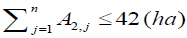
| SC2 | 0.06 | 1.229 | 0.01 | 0.35 | 0.25 | 0.25 | 0.5 | 3000 | 42 |
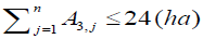
| SC3 | 0.034 | 1.068 | 0.01 | 0.3 | 0.2 | 0.2 | 0.4 | 650 | 24 |
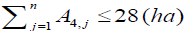
| SC4 | 0.06 | 1.229 | 0.008 | 0.35 | 0.25 | 0.25 | 0.5 | 1150 | 28 |
Estimation of seepage from canal
General framework: The general framework that was used for the estimation of seepage from canals in this study area is illustrated in (Figure 6). The historical canal data such as dimension of canal, soil type on which the canal was constructed and soil hydraulic conductivity underlying the canal foundation were used to estimate water loss through seepage. Moreover, data was collected on existing canal cracks, weed growth within the canal and canal leakage.

Figure 6. Depiction of ponding test method.
Canal rating and selection for a ponding test: In most cases, canals are pre-selected for testing because of known problems and rehabilitation plans. A more systematic approach is to rank canals using certain parameters. Some of the canal parameters that can be used to prioritize the selection of canals for ponding test were types of canals that can be either lined or earthen (annual use/area served and current conditions of the canal such as visible leaks, water and vegetation in drain ditch, and vegetation. The canal reach selection for ponding was carried using the information in (Table 7).
| Type | Level of canal | General condition | Cracks/holes (lined only) |
vegetation growing in canal |
|---|---|---|---|---|
| main canal | Mc1 | 2 | 1 | 0 |
| secondary canals | Sc1 | 2 | 1 | 1 |
| Sc2 | 2 | 2 | 1 | |
| Sc3 | 3 | 2 | ||
| Sc4 | 3 | 2 | 1 | |
| Rating scale | General condition
|
1.Hairline 2.Pencil-size 3.Large |
|
|
The ponding test method: Measuring seepage loss rates is one of the best ways to prioritize canals for maintenance and rehabilitation and determine the effectiveness of canal improvements quantified through pre- and postrehabilitation testing. There are several methods of estimating and measuring seepage losses from canals. The accuracy of these methods depends on the type of flow meter and measuring technique used the size of the canal and the volume of water. The ponding test method is considered the most accurate, and is often used as a standard of comparison for other methods In this method two ends of a canal segment are closed or sealed (usually with earthen dams) to create a ponded pool of water The change in water level is measured over 24 to 48 hours and was used along with the canal dimensions to calculate the seepage loss rate from the canals. Ponding test is classified as either “seepage loss tests” or “total loss tests” depending on the characteristics of the canal segment and the presence of leaking valves, gates and other structures. Seepage loss tests measure the seepage losses through the bottoms and sides of canals. Short canal segments are often used to avoid valves, gates or other structures that can leak. Thus, all water loss is due to seepage through a canals bottom and sides. Total loss tests were conducted in canal segments that contain valves, gates and other structures that might contribute to the losses measured. It may be important to account for losses from leaky control structures when considering canal improvements, but these types of leaks are often hard to notice and difficult to measure separately from canal seepage. In this study, the seepage loss tests were done for obtaining optimal canal dimension.
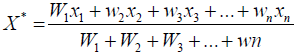
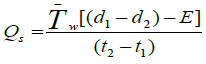
Calculation of seepage loss rate: According to the upstream and downstream of the test section were closed and water was filled in to the section to start reading the change in water level in the section. During this time, three or more staff gauge was required for reading the change in water level. The staff gauges were located at both ends of the section and at the middle of the section in order to overcome the water level fluctuation error during the period of extreme wind condition. In this study, the test was made for two days and after accounting for evaporation, the calculation of the seepage loss rate was done according to the method by as shown in Equation 3.
 (3)
(3)
Where: Qs = seepage rate (m3/se),
• w average water surface top width between times t1 and t2 (m),
• L = length of channels between dams (m),
• d1 = water level at time t1 (m),
• d2 = water level at time t2 (m),
• E = evaporation depth between time t1 and t2 (m),
• P = precipitation depth between time t1 and t2 (m),
• t1 = time at first measurement of water level (sec),
• t2 = time at subsequent measurement of water level (sec)
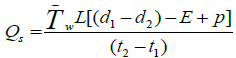
In principle, consideration for precipitation, evaporation, and diversion from and to the test reach is important. However, the study period and method of canal reach selection for ponding test matter for considering all these factors. In this study, since the study period was during dry season the consideration of rainfall was not important. Furthermore, the canal reach for the test section was not included any turnout for diversion purpose. Therefore, the formula to determine the seepage rate without considering precipitation was given in Equation 4.
 (4)
(4)
(Figure 6). Below describes the seepage ponding test measurement procedure.
In Equation 4, the loss due to evaporation is incorporated but most of the time the evaporation from small canals is very small and can be neglected from the calculation of seepage. Pointed out that the evaporation of water from exposed surface of the canal ranges from 0.25 to 1% of the total canal discharges and most of the time ignored from the calculation of seepage loss. According to the evaporation loss in irrigation networks is generally not taken into consideration because it is only 0.3% of total stream loss, whereas second. The procedure for field seepage measurement was depicted in (Figures 7 and 8). Following the above procedure, results of seepage loss rate from all secondary canals were summarized in (Table 8).

Figure 7. Estimation of seepage losses from irrigation canals using ponding test method.

Figure 8. Comparisons between crop demand and designed discharge first crop pattern.
| Canals | Depth (m) | Time (hrs.) |
Top width (m) | length (m) | Qs (m3/s) |
|---|---|---|---|---|---|
| Main canal(d1) | 0.5 | 48 | 0.4 | 150 | 3.5E-05 |
| main canal (d2) | 0.4 | - | - | - | - |
| Sec. canal 1(d1) | 0.3 | 48 | 0.2 | 317 | 3.6E-05 |
| sec. canal 1(d2) | 0.2 | - | - | - | - |
| sec. canal 2(d1) | 0.45 | 48 | 0.30 | 3000 | 1.56E-03 |
| sec. canal 2(d2) | 0.15 | - | - | - | - |
| sec. canal 3(d1) | 0.5 | 48 | 1.0 | 650 | 1.57E-03 |
| sec. canal 3(d2) | 0.08 | - | - | - | - |
| sec. canal 4(d1) | 0.45 | 48 | 0.28 | 1150 | 1.8E-03 |
| sec. canal 4(d2) | 0.10 | - | - | - | - |
Optimization model
Description of scenarios of optimization model: The Net benefit maximization model has formulated by using Linear-Programming model under different scenarios. Net benefit means the amount of profit after all constraint of cost have selected optimally. The aim is to maximize profit by applying available water optimally and allocating the land to different crop. The scenarios considered are; Scenario-I, that investigated for the full design discharge in canal to explain how it is beneficiary if the canal design well maintained and without any damage. Scenario-II developed under design discharge less seepage discharge to investigate the effect of seepage loss on crop yield reduction and benefit. Scenario- III, developed under optimized canal discharge and minimum seepage to investigate how much benefit increased due to minimized loss. Note that in scenario I and II, all canal dimensions and proposed area under each canal is according to existing condition except their discharge. The third scenario formulated based on optimized canal dimension and minimum seepage as well as with existing command area under each canal. The last and the fourth scenario have formulated based on allocation of required area proposed in this research and other conditions are similar to third scenario. Comparing all of the scenario, which will compete among different constraints and giving suggestion for farmers and irrigation department of the study area is the end result of this paper. While applying this scenario many major portion (98.37%) is due to seepage. In this study, it was difficult to measure the evaporation loss from the canals due to the following reasons; (1) the measuring instrument was not available during the data collection. (2) There is no convenient empirical formula to estimate evaporation even if the empirical formula used the instrument that used to measure the surface water temperature is also hard to get by rent. (3) As described in several literatures evaporation from small canals is small and could be neglected. Hence, the formula to calculate seepage from canals without considering evaporation loss was shown in Equation 5 below.
 (5)
(5)
In Equation 5, seepage discharge was calculated in cubic meter per data such as design discharge of every canal in the network, original canal dimension such as bed width and depth, length of each canal in the network, area allocated to each branch canals, production rate of crop, sailing price of the crop, production cost, and climate data, are required as secondary data. The data such as seepage rate, the existing canal dimension, the permeability of the soil underlying canal bottom at existing condition will be required as primary data.
As described in the above paragraph, the 1st scenario is the maximization of net profit having full design discharge with maximum design dimension of canal assuming if seepage is negligible in canals. The 2nd scenario consider the only possible available water by reducing the seepage discharge from the original design discharge with existing condition without minimization of seepage in canals. The 3rd scenario apply the minimization of seepage for optimum dimension such that the discharge of each canal in the network is adjusted with minimum seepage discharge and the 4th scenario use optimum discharge and optimum canal dimension similar to scenario III but the area under each secondary canals proposed to be 6 ha, 38ha, 22ha and 34ha for sc-1, sc-2, sc-3 and sc-4 respectively instead of 6ha, 42ha, 24ha and 28ha for sc-1, sc-2, sc-3 and sc-4 respectively. In order to perform this work, the step wise process will be applied to reduce the complexity of optimization problem such that the optimization of seepage and canal dimension is performed for the third and fourth scenario of benefit optimization using Lagrange optimization model. The seepage equation along the wetted perimeter of the canal will be formulated according to liu dong to select optimal dimension of canals considering seepage losses from canals. This selection will be performed by multiplying the non-dimensional bed width and depth of canal with length scale provided in the model such that seepage will be reduced along with reduction in flow depth and this idea were pointed out by adarsh.
For benefit maximization, the simple linear programming (LP) model formulated by considering the available water at each scenario in the first step as one of the resource constraints and such that considering the area allocated for each canal and competition crops under this area as a decision variable of this model. As explained above the constraints are available water, maximum and minimum planting area, total area, including the constraint related to production cost and man power. In order to utilize the water resources reasonably, to match water supply and requirement and reach the maximum economic benefit, the optimum crop pattern for the network of branch canal was first determined as pointed out by Each of the considered scenarios described here after.
Scenario - I under full design discharge (Qd): In this scenario, the linear optimization model formulated under full design discharge by assuming if the canal is without any damage and loss due to seepage is nil. This scenario is important for awareness creation for design engineer during the construction work of canals in terms of lining material selection to minimize the loss of water to accepted level pointed out that 99% perfect lining of canal can stop the loss of water due to seepage and increase the economic benefit of crop production. So that in this scenario, the canal discharge is equal to the design discharge and the canal dimension also the same to existing dimension and the value of discharge and velocity of water flow and other related dimension taken from (Table 4).
Scenario - II under design discharge with existing seepage discharge (Qd-qs): This scenario is nothing but existing condition. Under existing condition, there are many problems in canal such as canal leakage, percolation of water through canal bed and depth; however, the linear programming formulated for existing available discharge by deducting the amount of water lost due to seepage from design discharge. The amount of seepage in this case is determined from the field measurement using ponding method. In this scenario, the aim is to see and quantify how much economic benefit is lost due to the loss of water. The linear programming allocate small hectares of land for small amount of available water this shows that the effect of less water delivered to the command due to loss. In this case, the optimization problem formulated using (Tables 6 and 8). By deducting seepage discharge from design discharge and the result is available discharge. From the result of this scenario, one can understand the economic value of single droplet of water and can give self-suggestion for the problem of seepage.
Scenario - III under optimum canal discharge Opt [Qd]: This scenario dealt with minimization of seepage, optimum canal dimension, and optimum discharge. During this year (i.e.2019/2020), the irrigation bureau of kiltie Awlalo Woreda limited the command area of the korir scheme to 26 ha of land out of 100 ha due to highly shortage of water. As well as they were limited the production of crop to tiff only since the water requirement of teff is less compared to other crops. Under this scenario, the aim is to see the amount of land allocated for irrigation under different crop and its economic benefit. One can suggest either to continue with the existing condition with low benefit or adopting the cropping pattern given by linear programming. In this scenario the model, use the optimal value of canal dimension and optimal design discharge. Minimizing seepage means minimization of flow area since seepage losses occur on the flow perimeter. The optimal design of canals for minimum seepage loss involves the estimation of seepage loss subject to the uniform flow constraints. The exact analysis of seepage loss from canals is quite complex. In the present study the simplified and approximated expressions proposed by Vishnoi, Ram, Ram Prakash and Ravi Saxena. Adopted to formulate the optimization model for minimum seepage loss designed irrigation canals. The development of optimization model has presented below. The steady seepage loss from an unlined or a cracked lined canal in a Homogeneous and isotropic porous medium expressed as in Equation 6.
qs = KP (6)
Where, qs is the seepage discharge per unit length of channel, m2/s; K is the hydraulic conductivity of the porous medium, m/s; P is the wetted perimeter, m. Equation 6 can be rewritten for rectangular section as follows in Equation 7.
qs = (b+2yn) (7)
Since the channel type of the study area is rectangular, we can only focus on rectangular section
Objective Function: The objective of the above model can be considered as the minimization of non-dimensional wetted perimeter multiplied by a permeability of underlying canal material. It has been proved that the solution of minimum wetted perimeter and minimum flow area problems, would result in the same values of section variables. This means that the solution of minimum wetted perimeter or minimum flow area problems, considering the uniform flow equation as the sole constraint, will result in the same values of section variables.
Minimize A = Minimize P (8)
Minimize qw = KP (9)
The terms of this model, all variables are all in dimensional forms. In order to easily trace the effects of variables on the model, the above equations put into non-dimensional forms. This conversion has done by defining a length scale, λ as follows.
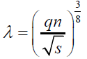 (10)
(10)
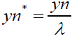
Non-dimensional Forms
 (11)
(11)
 (12)
(12)
 (13)
(13)
 (14)
(14)
Using the above expressions, the final optimization model in nondimensional form can written as follows,
min imize qw = k (b* + 2yn*) (15)
 (16)
(16)
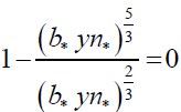
The solution of the above optimization model for each channel type will result in the optimum values of non-dimensional bottom width, flow depth, and channel radius for the case of no additional cost term. These values of section variables will form the boundary conditions for numerical analysis. In order to solve the above optimization problem, the objective and the constraint functions combined to form an augmented function. The general structure of the augmented function, ɸ is as follows,
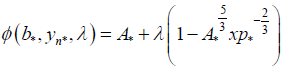 (17)
(17)
 (18)
(18)
Where, λ = a Lagrange multiplier
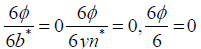
Since the value of constraint function (Equation 16) at the optimum solution should equal to zero, the optimum points of augmented function will not differ from the optimum values of original objective function. By using the principles of differential calculus, the augmented function and the conditions to be satisfied for rectangular channel type given in appendix 1. According to the channel type considered, the above equations are solved simultaneously for the optimal values of non-dimensional section variables. The optimum values of bottom width, b*, normal depth, yn* can be easily computed by multiplying the corresponding optimum non- dimensional values by the length scale, λ. in appendix 1
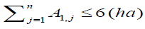
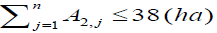
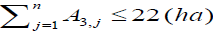
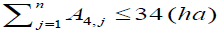
Scenario - IV optimum benefit under new proposition of command area to each canal: In scenario I, II and III the command area under each canal is according to existing condition, which is 6ha, 42ha, 24ha, and 28ha to Sc-1, Sc-2, Sc-3 and Sc-4 respectively. In this scenario the new command area is proposed to each canal, this condition may use to compensate the deficiency of canal discharge to crop water need and the loses that are not included in this study such as field application loss and evaporation losses from both canals and command area. Therefore, the new proposed area to each canal is 6 ha, 38 ha, 22 ha, and 34 ha to Sc-1, Sc-2, Sc-3, and Sc-4 respectively. This scenario uses optimum discharge, minimum crop pattern and optimum canal dimension similar to scenario III except new proposition of command area.
Cropping pattern selection: In this study, three major and four supplementary crops were identified to formulate LP model. Those considered as major crops are Pepper, Tomato, and Onion while those considered as supplementary crops are Cabbage, Spinach, Potato and Carrot. The organization of crop pattern was according to their market price, water requirement and social demand. During the study period (2019-2020) the observation of command area and informal discussion with farmers of the study area, indicate that Cabbage can be replaced by Spinach and Potato by carrot in terms of their use in food sources. Moreover, Spinach and Carrot needs less water relative to cabbage and potato. In the model formulation, Pepper, Tomato and Onion were considered in all scenarios and in all crop patterns since they considered as high value crops for this particular irrigation scheme. The supplementary crops were considered as crop pattern-I and crop pattern-II when cabbage and potato considered and spinach and carrot considered respectively.
Duty of crops: Duty is defined as the area irrigated by a unit discharge of water flowing continuously for the duration of the base period of a crop and larger areas can be irrigated if the duty of the irrigation system is improved. The duty is measured in hectares per cubic meter per second and depends on the crop, Type of soil, Irrigation and cultivation methods, climatic factors, and channel conditions. In this thesis work the duty of water were calculated in CROPWAT 8.0 window. The input data for the calculation are climate data, soil data, crop data (their growth stage, root depth, crop coefficient, and yield response factor) collected from different sources. Climate data such as rainfall, maximum and minimum temperature, wind speed, relative humidity and sunshine hours were collected and analyzed as discussed in section 3.2.2 above. The soil data such as soil types of the command area used for the calculation of duty of water for the input of CROPWAT software obtained from Satya, p. Garg and A. S. Chawla [9]. Data such as root depth, crop coefficient, yield response factor, deplation coefficient, growing date (stage length) are collected and amazed from (FAO, 2020) Finally all these data used as input for CROPWAT 8.0 software. The output data from the software are irrigation scheduling and scheme supply more over the duty of water is one of the output data form the model.
Formulation of linear programming (LP) model: The Korir irrigation scheme consists of four secondary canals under which deliver water to the command for five major dry season crops. For each secondary canal, the design command area was determined by GPS area calculator mobile application. The linear programming was formulated with the objective of maximization economic benefit from irrigation by existing canals. The decision variable is area allocated for a given amount of water under each branch canals to different competitive crop
Model objective function: The objective function of this LP model is benefit maximization with input variables of average yield of crop (Kg/ha), selling price of crop (ETB/Kg), production cost of crop (ETB/Kg). The total profit is the algebraic summation of these inputs and given as given in Equation 19.
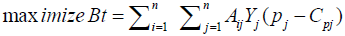 (19)
(19)
cpj = cf + cs (20)
Where;
Cpj = cost of production which includes cost of seed (Cs) fertilizer (Cf) in = (ETB/Kg),
Aij = area of crop j under branch canal i in (ha),
Yj = yield of crop j (Kg/ha), Pj =selling price (ETB/Kg),
Bt = the total benefit gained by irrigating five dry crops activity (ETB)
i= canal reference number, i=1, 2, 3, 4,
j= crop reference number, j=1, 2,3,4,5
Formulation of constraints
Constraints of command area under each secondary canal: The command area of each canal for Korir scheme was measured to be 6ha, 42ha, 24 ha and 28ha for secondary canal 1, 2, 3 and 4 respectively. The combined crop area irrigated per branch canal should be equal to or smaller than the total area irrigated by the canal and mathematically written as follows;
 (21a)
(21a)
 (22a)
(22a)
 (23a)
(23a)
 (24a)
(24a)
The above constraints were used to formulate the three scenarios under existing condition of command area but for the Scenario-IV (optimum benefit under new proposition of command area to each canal) the new proposed area and constraint is written as next section.
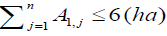
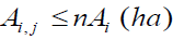
Constraints of proposed cropping pattern: The total area allocation proposed that during the canal rehabilitation of the scheme for pepper, cabbage, potato, tomato and onion should not be greater than 0.2, 0.15, 0.15, 0.25 and 0.25 of the given area under each canal respectively according to the agronomic feasibility report of Korir dam. However, the existing condition of irrigation scheme failed with deficit irrigation due to losses of water by different factors. Moreover, the command area was significantly reduced from 100ha to 26ha. To increase the command area to 100 ha new crops with minimum water consumption need to be proposed. Moreover, to reduce land without of irrigation, the allocation of the minimum area to be irrigated should be greater than 50% of the total command area. Mathematically
 (25)
(25)
Where;
A i, j = is the total area allocated for each crop under each branch canal
n = is the coefficient of cropping pattern, which represent the value of 0.1, 0.075, 0.075, 0.125 and 0.125 for pepper, cabbage, potato, tomato and onion respectively.
 (21b)
(21b)
 (22b)
(22b)
 (23b)
(23b)
 (24b)
(24b)
The above cropping pattern total sum is equal to 50 ha. This cropping pattern is the allowable minimum area irrigated during the lowest discharge in canal. The reason for deciding the half of total command area is the worded agriculture and rural development office recommend the farmers each year how much they must to irrigate based on the availability of discharge in reservoir. However, it is not profitable to recommend only based on the availability of water but also need to optimize the irrigation systems. Additionally the upper boundary of command area has given by the constraint of command area under each secondary canal as explained in equation (21-24a) and (21-24b).
Constraint of water supply: The water supplies always limited to the available discharge in canal based on the fluctuation of water level in storage reservoir. We know that there is inconvenience in storage reservoir to grow high water required crop. Therefore, it needs to search the crops that require minimum water and fulfill the social and market demand. In the study area during the study year, the single crop had recommended to farmers by worked as agriculture and rural development office because of shortage of water. Even though single crop irrigated it was not possible to irrigate total irrigable land (only 26ha of land irrigated Teff crop out of 100ha). Therefore, to tackle the problem of shortage of water and to irrigate all irrigable land, eight crops types were identified and their crop water requirement calculated using CROPWAT model in terms of their irrigation duty (l/s/h). After converting the unit of irrigation duty to (m3/s/ha), this duty multiplied to area allocated to each crop and this give discharge unit. Finally the discharge required by crop must less or equal to the optimum design discharge of a given canals and the constraint could be written mathematically in Equation 26.
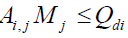 (26)
(26)
Ai,j = the area allocated to each crop under secondary canal i
Mj = maximum duty of crop j during growing season (m3/s/ha)
Qdi = discharge of canal (m3/se)
Constraints on seed cost: Farmers of the study area irrigate their land buying the crop seed from different agency and the cost of seed required per hectare of land given in table under economic data of section 3. Since the net benefit mean the different between cost and benefit of crop production, the total cost of seed need to irrigate allocated command area under each canal must be less than or equal with the cost of seed need to irrigate the total land designed for each canal and mathematically;
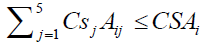 (27)
(27)
Where, CSj = Cost of jth crop seed per Ha in ETB, Aij = Area of jth crop under ith secondary canal in Study area in Ha, and CSAi = Total cost of seeds per entire CCA under each secondary canal in ETB.
Constraints on fertilizer cost: The constraint on the fertilizer cost also formulated similar to the seed costs. The total cost of fertilizer need to irrigate allocated command area under each canal must be less than or equal with the cost of fertilizer need to irrigate the total land designed for each canal and mathematically;
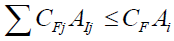 (28)
(28)
Where, CFj = cost of jth crop fertilizer per ha in ETB, Aij= Area of jth crop under ith secondary canal in Study area in Ha, and CFAi = Total cost of fertilizer per entire CCA under each secondary canal in ETB.
Irrigation duty of crops: Duty is defined as the area irrigated by a unit discharge of water flowing continuously for the duration of the base period of a crop and Larger areas can be irrigated if the duty of the irrigation system is improved. To determine the irrigation duty of different crop, climate data for 28 years has analyzed and incorporated in to CROPWAT 8.0 software with every crop characteristics, soil type, planting and harvesting date of each crop. CROPWAT software gives the output of crop water requirements. This requirement varies at different stages of the growth of the plant. The peak requirement must be obtained for the period of the keenest demand and the related irrigation duty (m3/s/ha) of each crop and these result tabulated in the (Table 9). The total irrigation duty of each crops used to determine the amount of water required for crops during their growing season. The maximum irrigation duty in the above table used to formulate the optimum water to allocate to each secondary canal sufficient to irrigate selected crops in the scheme and based on this discharge the optimum canal dimension also selected by using Lagrange optimization method minimizing the amount of seepage from canals.
| Month | Crops | |||||||
|---|---|---|---|---|---|---|---|---|
| pepper | cabbage | Potato | Tomato | Onion | Spinach | Carrot | Lettuce | |
| Dec | 1.30E-04 | 2.90E-04 | 2.30E-04 | 2.50E-04 | 2.40E-04 | 1.50E-04 | 1.50E-04 | 1.50E-04 |
| Jan | 3.60E-04 | 5.10E-04 | 5.00E-04 | 4.10E-04 | 5.10E-04 | 4.50E-04 | 4.20E-04 | 3.00E-04 |
| Feb | 5.90E-04 | 6.20E-04 | 6.80E-04 | 6.60E-04 | 6.20E-04 | 3.50E-04 | 6.20E-04 | 5.50E-04 |
| Mar | 6.80E-04 | 6.71E-04 | 3.20E-04 | 7.30E-04 | 6.80E-04 | 0.0E+00 | 3.80E-04 | 4.80E-04 |
| Apr | 3.40E-04 | 6.00E-05 | 0.0E+00 | 3.70E-04 | 6.50E-04 | 0.0E+00 | 0.0E+00 | 0.0E+00 |
| May | 0.0E+00 | 0.0E+00 | 0.0E+00 | 0.0E+00 | 1.60E-04 | 0.0E+00 | 0.0E+00 | 0.0E+00 |
| Total | 2.10E-03 | 2.15E-03 | 1.73E-03 | 2.42E-03 | 2.86E-03 | 9.50E-04 | 1.57E-03 | 1.48E-03 |
Scenario I Optimal benefit and area allocation to each crop using design discharge
Scenario I crop pattern I: Scenario I crop pattern I investigate that the effect of selected crop that aim to full fill the social and economic need of the society of the study area on the design discharge and net benefit obtained from them. The crops types selected for this condition are Pepper, Cabbage, Potato, Tomato, and Onion. Under this scenario, the aim is to investigate how much the design discharge is sufficient to irrigate the selected crop, the benefit from crop production, and the area allocated to each crop under each secondary canals. The scenario is under full design discharge that means when the loss due to seepage is not considered. In addition, different crop also incorporated in the model since different crop have different crop water requirements. Under each scenario, it needs to comparison between the first crop and second crop in terms of their benefit, area allocation and their water needs under each secondary canal. The result shows that under design discharge or under full discharge, the proposed cropping pattern and allocated area for each crop under each secondary canal irrigate proposed area except secondary canal 3 with maximum net benefit of 114,644,504.03 ETB from 99.9 ha of land out of total irrigable lands. The designed discharge under the assumption of any loss can irrigate 99.9ha of the irrigable land by saving minimum percentage of water from crop water demand and the result shown as following figure. Under this scenario, for all canals the design discharge greater than crop demand except in third secondary canal for example for secondary canal 1, 2, 3, and 4 the percentage of saved discharge is 35%, 1%, 0%, and 34% respectively. The largest difference occurred in the secondary canal 1 and 4 is because of while they serving small area but their design capacity relatively large when compared with secondary canal 2 and 3. More over in secondary canal 2 and 3 the design discharge is under warning of deficit irrigation even if it is enough to irrigate proposed area of land, it is risky in case of loss due to application, seepage and evaporation. This scenario is just imaginary because it assumes that full design discharge without any loss, even though there are many losses in irrigation system due to conveyance, seepage, application and operation (Table 10).
| Canals | Area of each Crops (ha) | Obj.Func (ETB) | ||||
|---|---|---|---|---|---|---|
| Pepper | Cabbage | Potato | Tomato | Onion | ||
| 1 | 0.6 | 0.45 | 0.45 | 3.75 | 0.75 | 68,84,421.00 |
| 2 | 4.2 | 3.15 | 3.15 | 26.25 | 5.25 | 4,81,90,947.00 |
| 3 | 2.4 | 1.8 | 1.8 | 14.93 | 3 | 2,74,41,838.03 |
| 4 | 2.8 | 2.1 | 2.1 | 17.5 | 3.5 | 3,21,27,298.00 |
Scenario I crop pattern II: Scenario I crop pattern II is when some crops from crop pattern I replaced by other crops. From the first case, pepper, Tomato, and Onion are the minimum requirement, which farmers need during irrigation season because these crops have high value when compared to other. Therefore, crop pattern II governed by Pepper, Spinach, Carrot, Tomato, and Onion. The result shows that, allocation of land in the second case is greater than the first crop pattern by 0.1ha this is because the crop water demand for spinach and carrot further less than that of cabbage and potato. Therefore, the linear programming allocated the acreages up to the maximum available land since design discharge is greater than crop water demand. However something different from the first cropping pattern, which is net benefit, obtained from each crop under each secondary canal; this is nothing but the different in the market price of each crop. From the result of (Table 11). The total net benefit is 112,339,000.00 ETB, which is lower by 2,305,504.03 ETB (2%) from the first condition. The designed discharge without any loss and by exchanging cabbage with spinach and potato with carrot can irrigate all of the irrigable land by saving minimum percentage of water from crop water demand and the result shown in (Figure 9).
| Canals | Area of each Crops (ha) | Obj.Func (ETB) | ||||
|---|---|---|---|---|---|---|
| Pepper | Spinach | Carrot | Tomato | Onion | ||
| 1 | 0.60 | 0.45 | 0.45 | 3.75 | 0.75 | 67,40,340.00 |
| 2 | 4.20 | 3.15 | 3.15 | 26.25 | 5.25 | 4,71,82,380.00 |
| 3 | 2.40 | 1.80 | 1.80 | 15.00 | 3.00 | 2,69,61,360.00 |
| 4 | 2.80 | 2.10 | 2.10 | 17.50 | 3.50 | 3,14,54,920.00 |

Figure 9. Comparisons between crop demand and designed discharge second condition.
Under this scenario unlike to first cropping pattern, for all canals the design discharge greater than crop demand for example for secondary canal 1, 2, 3, and 4 the percentage of saved discharge is 37%, 3%, 3%, and 36% respectively. The largest wsater saving occurred in the secondary canal 1 and 4 is because of while they serving small area but their design capacity relatively large when compared with secondary canal 2 and 3. This scenario is under lower risk compared to the first scenario in terms of deficit irrigation with net benefit lower than the first condition by 2% (2,305,504. 03ETB). The reduction of net benefit due to the only reason of selling price of crops and production rate of carrot (i.e. Selling price of carrot is 20ETB/kg but that of potato is 25ETB/kg and the production rate of carrot is 90quintal/ha while that of potato is 200quintal/ha).
Scenario II Optimal benefit and area allocation to each crop considering measured seepage loss
Scenario II cropping pattern I: The result of scenario II cropping pattern I from linear programming are shown in (Table 12) and discussed. This scenario used to analyse the allocation of land and the maximum benefit under the reduced canal discharge capacity due to the effect of seepage loss. In this scenario, the model allocates only 38ha of land under the 2nd secondary canal out of 42ha irrigable land and allocate 19. 5ha of land out of 24ha under 3rd secondary canal that means the investigation shows that to allocate 42 ha and 24it needs additional water 10% and 20% on available discharge in 2nd and 3rd secondary canal respectively. In another words 10% of design discharge has lost by seepage. Beside this while, it serving larger area than the third secondary canal, which is earthen canal, serving only 24 ha the canal is more saviour than the third secondary canal because it loses 20% of design discharge to irrigate the area contained under it.
| Canals | Area of each Crops (ha) | Obj.Func (ETB) |
||||
|---|---|---|---|---|---|---|
| Pepper | Cabbage | Potato | Tomato | Onion | ||
| 1 | 0.6 | 0.45 | 0.45 | 3.75 | 0.75 | 68,84,421.00 |
| 2 | 4.2 | 3.15 | 3.15 | 22.22 | 5.25 | 4,27,70,119.97 |
| 3 | 2.4 | 1.8 | 1.8 | 10.55 | 3 | 2,15,43,624.33 |
| 4 | 2.8 | 2.1 | 2.1 | 17.5 | 3.5 | 3,21,27,298.00 |
In general, considering seepage loss, the model only allocates 91.5ha out of 100 irrigable lands even selecting vegetable cropping pattern. Moreover, the related irrigation benefit under this scenario is 103,325,463.30 ETB from all land under all canals. Similarly, the related net benefits under each secondary canal tabulated in (Tables 12 and 13). Above Moreover due to seepage we can lose 11,319,040.73 ETB (i.e.10% less benefit) comparing the design discharge of scenario I first condition. In addition, the comparison of crop water demand and canal discharge discussed in the following graph; From (Figure 10). We can understand that model, allocate only up to maximum design capacity of canal in second and third secondary canals. In those two secondary canals, we can see that the amount of water loss is maximum compared to the first and fourth secondary canals. Due to seepage loss in the canal the model, allocate 38ha out of 42ha and 19.5ha out of 24ha loosing 5,420,827.03 ETB and 5,898,213.70 ETB (i.e.11% and 21%) from second and third secondary canal respectively when compared to first scenario 1st crop pattern. The depiction of allocation of command area with respect to discharge has shown in (Figure 11).
| Canals | Area of each Crops (ha) | Obj.Func (ETB) | ||||
|---|---|---|---|---|---|---|
| Pepper | Spinach | Carrot | Tomato | Onion | ||
| 1 | 0.60 | 0.45 | 0.45 | 3.75 | 0.75 | 67,40,340.00 |
| 2 | 4.20 | 3.15 | 3.15 | 23.43 | 5.25 | 4,33,87,248.12 |
| 3 | 2.40 | 1.80 | 1.80 | 11.24 | 3.00 | 2,18,96,268.99 |
| 4 | 2.80 | 2.10 | 2.10 | 17.50 | 3.50 | 3,14,54,920.00 |

Figure 10.Comparisons between crop demand and available discharge scenario ii first condition.

Figure 11. Allocation of command area with respect to available discharge first condition.
Scenario II Crop pattern II: In this scenario, the discharge available in the canal considered the same with scenario II first condition but the types of crop considered is same with scenario I second case. This condition is aim to investigate whether crop water requirement is match with existing condition of canals or not. In this condition, the model only allocates 1.9ha of additional command area than the first condition of scenario II by exchanging cabbage with spinach and potato with carrot. In general, considering seepage loss, the model only allocates 93. 4ha out of 100ha irrigable lands even selecting vegetable cropping pattern with minimum crop water requirements. Moreover, the related irrigation benefit under this scenario is 103,478,777. 11 ETB from all land under all canals. Comparing with scenario II first condition, we have the benefit of 153,313. 81 ETB in this scenario (i. e. Scenario II second condition gives 0.15% more benefits than scenario II first condition). However, when compared with scenario II first condition the reduction of net benefit occurred by 2% in secondary canal 1 and 4. The overall discussion about the effect of available water and selling price of crops on crop water need, area allocation and net benefit summarized in the following figure from (Figure 12). Above we can conclude that, in 2nd and 3rd secondary canal zero amount of water has saved in canal from crop demand this shows that there is no amount of water required to compensate evaporation and field losses during irrigation. However, it is still surplus in 1st and 4th secondary canals by 37% and 33% more discharges available than crop demand. Moreover, the canal could be safe in case of other losses such as evaporation and field losses. Additionally, the effect of available water on area allocation has discussed in the following figure.

Figure 12.Comparisons between crop demand and available discharge scenario ii second condition.
As we understand from (Figures 13 and 14). Even though model allocate 1.2ha and 0.7ha of additional land for 2nd and 3rd secondary canal when compared with scenario II first condition we also see that the reduction of net benefit by 144,081.00 ETB and 672,378. 00 ETB in 1st and 4th secondary canal command in other side. The increments of land allocation in second and third secondary canal and the decrement of net benefit in first and fourth secondary canal command area is due to less crop water need of Spinach and Carrot compared with Cabbage and Potato and less selling price and production rate of Carrot compared with that of Potatos. Even though there is reduction of net benefit in first and fourth secondary canal command area, the result of scenario II second condition is justifiable than scenario II first condition because the net benefit of the second condition is larger by 0.15% than that of first condition

Figure 13.Allocation of command area with respect to available discharge second condition.

Figure 14.Comparisons between crop demand and designed discharge scenario iii first crop pattern.
Scenario III: Optimum allocation of command area and net benefit under optimum (minimum) result of seepage and section variables
The result of scenario I and II above is based on the dimension of canals given in (Table 6) of section 3. The scenario I is based on design discharge without considering seepage loss. The amount of seepage loss measured from canals using pond method for this research. This value was used in the second scenario to investigate the effect of canal seepage on the benefit of crop production. The seepage loss in canal depends on the wetted perimeter of canal that is maximum when the canal dimension is maximum. In canal design, it is good if the dimension of canal fixed according to crop water demand and carefully selected taking into account the section factor of canals. Now in the third scenario, the model run under minimum seepage losses with selected cropping pattern. The best dimension of canal that minimizes seepage value selected by Lagrange method and discussed in the following section. After defining the model variables, the next step is to specify the solution options. Under the “Solver Options” menu, one has the chance of setting the parameters, which control the precision, and the time spent for the solution. These parameters are maximum iteration time (in seconds), maximum iteration number, precision, tolerance and convergence. The default values used in this study are 100, 1000, 0.00000001, 5%, 0.0001, respectively. Since all the inputs and model options are specified, the software can be executed by just clicking the “Solve” button. Here, it should be noted that the system is solved for the non-dimensional optimum values of section variables. Then after the optimum section variable will be, obtain by multiplying the optimum non-dimension section variable with Lagrange multiplier (Lambda value) and the result of optimum value of section variable listed in the following table. In the result of (Table 14). The value of seepage from optimization differs from that of measured from field by ponding method. In addition, at the same time the canal dimension from optimization with respect to given design discharge is also differ from actual dimension. To see their different refer (Tables 8 and 14). The amount of discharge saved in optimization method from Sc-1, Sc-2, Sc-3, and Sc-4 is 20%, 68%, 86%, and 69% respectively when compared to the actual seepage losses.
| Canal | Q des (m3/se) | K (m/s) | lambda | bed width (b) | Normal depth (Yn) | qw (m2/s) | Length (m) | qw (m3/s) | Qopt (m3/se) |
|---|---|---|---|---|---|---|---|---|---|
| Sc-1 | 0.0132 | 1.00E-06 | 0.104 | 0.19 | 0.10 | 3.81E-07 | 317 | 1.21E-04 | 0.013 |
| Sc-2 | 0.06 | 1.00E-06 | 0.183 | 0.34 | 0.17 | 6.71E-07 | 3000 | 2.01E-03 | 0.058 |
| Sc-3 | 0.034 | 2.30E-06 | 0.161 | 0.29 | 0.15 | 1.36E-06 | 650 | 8.82E-04 | 0.033 |
| Sc-4 | 0.06 | 1.00E-06 | 0.191 | 0.35 | 0.18 | 7.00E-07 | 1150 | 8.05E-04 | 0.059 |
Scenario III cropping pattern I: In this scenario, crop types considered same to scenario I crop pattern I and the only different is optimum discharge, which is the different between design and optimum seepage value from optimization model, is used. Using minimum seepage losses obtained from optimization model the linear programming allocate 98. 1 ha of land out of 100 ha using the first cropping pattern such as pepper, cabbage, potato, tomato, and onion. This value is larger than the 2nd scenario of both conditions when actual seepage reduced from design discharge with actual canal dimension. In addition, the area of each crop allocated under each branch canal with total net benefit under each branch canal tabulated in the (Table 15). Above the total net benefit from all allocated command area and respective crop is 112,172,783. 85 ETB. The result is more appreciable when compared to second scenario of first and second condition with around 8,847,320.55 ETB and 8,694,006. 74 ETB more benefit respectively
| Canals | Area of each Crops (ha) | Obj.Func (ETB) | ||||
|---|---|---|---|---|---|---|
| Pepper | Cabbage | Potato | Tomato | Onion | ||
| 1 | 0.60 | 0.45 | 0.45 | 3.75 | 0.75 | 68,84,421.00 |
| 2 | 4.20 | 3.15 | 3.15 | 25.10 | 5.25 | 4,66,40,822.71 |
| 3 | 2.40 | 1.80 | 1.80 | 14.24 | 3.00 | 2,65,20,242.14 |
| 4 | 2.80 | 2.10 | 2.10 | 17.50 | 3.50 | 3,21,27,298.00 |
From the result of scenario III first condition, we can see that the effect of seepage on crop water requirement has minimized and only 1.9ha of land has left from irrigation out of total command area and 1.8ha has left from Scenario I first condition. Even though there scarcity of water in secondary canal 2 and 3, 34% and 33% of water is surplus in the secondary canal 1 and 4 respectively. The effect of available water on area allocation has shown in the following figure discussed as bellow. From graph shown in (Figures 15 and 16). Above the allocation of area increased by 3.3ha and 3.7ha for 2nd and 3rd secondary canal when compared with scenario II first condition and by 1.6ha and 3.0ha for 2nd and 3rd secondary canal when compared with scenario II second condition. More over this value shows that the linear programming model allocate better net benefit when seepage from canal minimized and with optimum dimension and optimum discharge. However, the shortage of discharge in secondary canal 2 and 3 still not solved similar to these scenario I and II.

Figure 15. Allocation of command area with respect to available discharge first condition.

Figure 16.Allocation of command area with respect to available discharge under scenario III second crop pattern.
Scenario III cropping pattern II: Under optimized canal dimension and minimum seepage loss, by exchanging crop to each other similar to scenario I&II the result of net benefit from crop production and allocation of command area for each crop under each branch canal tabulated, and shown in (Table 16 and 17). The above result indicate that the effect crop water requirement on available optimum discharge and net benefit. This effect is positive effect on both area allocation and net benefit in both secondary canal 2&3 (i.e. Model allocate all required area for secondary canal 2 and 23. 9ha out 24 ha for secondary canal 3) with total net benefit of 112,250,526.79 ETB with command area of 99.9ha of land. Comparative to scenario III first condition, this scenario generate 77,742.94 ETB (i.e.0.1percentage) more benefit and allocate 1.8ha of additional command area. The replacement of cabbage with spinach and potato with carrot possibly irrigate 42ha of land with available optimum discharge of 0.058 m3/se under secondary canal 2 and 23.9 ha of land with 0.033m3/se under secondary canal 3. In general, the following graph briefly expresses this concept as follows. This scenario result in similar allocation of command area with scenario I first condition but the net benefit of this scenario has reduced by 2% from all secondary canal command area. More over this reduction is due to the lower selling price and production rate of carrot crop in the model (Figure 17).
| Canals | Area of each Crops (ha) | Obj.Func (ETB) | ||||
|---|---|---|---|---|---|---|
| Pepper | Spinach | Carrot | Tomato | Onion | ||
| 1 | 0.60 | 0.45 | 0.45 | 3.75 | 0.75 | 6,740,340.00 |
| 2 | 4.20 | 3.15 | 3.15 | 26.25 | 5.25 | 47,182,380.00 |
| 3 | 2.40 | 1.80 | 1.80 | 14.93 | 3.00 | 26,872,886.79 |
| 4 | 2.80 | 2.10 | 2.10 | 17.50 | 3.50 | 31,454,920.00 |
| Canals | Area of each Crops (ha) | Obj.Func (ETB) | ||||
|---|---|---|---|---|---|---|
| Pepper | Cabbage | Potato | Tomato | Onion | ||
| 1 | 0.60 | 0.45 | 0.45 | 3.75 | 0.75 | 68,84,421.00 |
| 2 | 3.80 | 2.85 | 2.85 | 23.75 | 4.75 | 4,36,01,333.00 |
| 3 | 2.20 | 1.65 | 1.65 | 13.75 | 2.75 | 2,52,42,877.00 |
| 4 | 3.40 | 2.55 | 2.55 | 21.25 | 4.25 | 3,90,11,719.00 |

Figure 17. Comparisons of optimum discharge and crop water demand for scenario IV first condition.
In general, in all scenarios, the design discharge of Sc-1 and Sc-4 is greater than their command area and crop water demand of selected crop while in secondary canal 2&3 the design discharge lack to fill the crop demand and irrigate command area allocated to them. This unfitting may be solved by reducing the command area from secondary canal 2&3 and adding to the secondary canal 1 and 4. However, from geographic condition of irrigation scheme, it is not possible to expand the command area under secondary canal 1(Sc-1) because the command area was separated from by small forest and natural drainage, which is not economical to deliver through these obstacles. In addition the area under secondary canal 2, 3 and 4 constructed in the same area and the 2nd secondary canal deliver water starting from the secondary canal 1 up to Endasillassie street around 3Km distance. By considering these conditions, we can implement additional scenario to solve the slack in secondary canal 2 and 3 and surplus of secondary canal 4. As stated in the above paragraph the surplus of secondary canal 1 can only be solved through operation of canal system according to command area and crop water requirement. As we can understand from all scenario, to command 6 ha of land and to obtain maximum benefit from the selected cropping pattern the model allocated 0.009m3/se of discharge during maximum crop water demand and 0.008m3/se during spinach and carrot replaced with cabbage and potato respectively. More over to save 34% of discharge applied to 6ha it needs to create awareness to the operator of dam and the farmers of this command area.
Scenario IV: Optimum allocation of area and net benefit under proposed command area under each secondary canal
Scenario IV cropping pattern II: In section 4.4-4. 5 the optimum value of area under each secondary canal and the maximum net benefit searched in the combination of existing area under each canal, proposed cropping pattern and existing design discharge. Different combination of these variable produced different optimum result of area and net benefit. As stated before, the existing area under each secondary canal; 6ha, 42ha, 24ha, and 28ha for Sc-1, Sc-2, Sc-3 and Sc-4 respectively. In this scenario, the proposed area under each secondary canal is 6ha, 38ha, 22ha, and 34ha for Sc-1, Sc-2, Sc-3, and Sc-4 respectively. The other condition such as cropping pattern, optimum dimension, and discharge is similar with scenario III and the result of optimization model discussed as below. The model allocates 10ha of pepper, 7.5ha of cabbage, 7.5 ha of potato, 62.5ha of Tomato and 12.5ha of Onion out of 100 ha for all canal with global maximum value of Net benefit (i. e. 114,740,350.00 ETB) irrigating 100 ha of land. In this programming the model, allocate total of proposed command area for each canal. When saying this, the model allocate 6 ha of land for Sc-1 with maximum benefit of 6,884,421.00 ETB, 38ha of land for Sc-2 with maximum benefit of 43,601,333. 00 ETB, 22ha of land for Sc-3 with maximum benefit of 25,242,877.00 ETB and 34 ha of land for Sc-4 with maximum benefit of 39,011,719.00 ETB. The model generates higher benefit in this scenario more than all provided scenario. This scenario similar with scenario I second condition in terms of area allocation that means both scenarios allocate 100 ha but the more benefit is obtained in the later scenario with about 2,401,350.00 ETB than scenario I second condition. Under this scenario the optimum discharge of all secondary canals are excess of their crop water demand. This condition is good to compensate the risk of water losses occur in evaporation and application of irrigation water and their allocation shown in figure below. From figure above, for all secondary canals the optimum discharge is greater than maximum crop water demand. More over 34%, 7%, 5% and 18% of discharge has saved from Sc-1, Sc-2, Sc-3 and Sc-4 respectively. The amount of discharge saved after optimization will be useful in case of losses due to evaporation and percolation in irrigation command.
Scenario IV cropping pattern II: This scenario investigate how much water saved when least crop water required crop used emplace of other crops. This condition similar with second condition of scenario I, II and III above in terms of crop types but other thing is similar with scenario III and scenario IV first condition in terms of optimum canal dimension, optimum discharge and proposed command area respectively. The model allocate total of 100ha land with relative maximum net benefit of 112,339,000.00 ETB. Additionally the allocation of command area is similar with scenario IV first condition however, the result of net benefit is less when compared to first condition. Under this scenario 54 even, we save premium amount of discharge, we losses the benefit of about 2,401,350.00 ETB when compared with scenario IV first condition. More over the distribution of discharge and allocation of land under this scenario has discussed as following (Figure 18). This scenario save 36% from sc-1, 10% from sc-2, 8% from sc-3 and 21% from sc-4 by allocating all irrigable land of the study area. The selection of best scenario must be done in the next section by comparing their area allocation, generated benefit and in terms of their saved discharge for the purpose of compensation of other losses. More over the social need must also incorporated in the selection of best scenario and the procedure has made in the next section

Figure 18.Comparisons of optimum discharge and crop water demand for scenario IV second condition.
Comparison and selection of best scenario
Comparison of area allocation to different crops under different scenarios: This section compares and tries to justify the cropping patterns developed under different scenarios. The graphical representation of the cropping patterns had presented in (Figures 19, 20 and 21). Show all scenarios with their respective allotment of command area. The first scenario is imaginary scenario, which allocate 99.9 ha when cabbage and potato incorporated in the model and allocate 100 ha when spinach and carrot replaced emplace of cabbage and potato. However, the allocation of total area increased linearly starting from scenario II to scenario IV with maximum allotment of command area at scenario IV. This increment is happen due to the linear increments of area allotted to tomato. For the purpose of selecting best scenario IV both condition allocate 100ha, however considering the social need of the study area scenario IV first condition is feasible to recommend to apply to study area.

Figure 19. Comparison of cropping pattern under different scenarios.

Figure 20.Comparison of net benefit under each canal command area under different scenarios.

Figure 21.Comparison of saved discharge under each canal command area under different scenarios.
Comparison of net benefit from different crops under different scenarios under each canal command: To identify best scenario that can produce maximum benefit under each canal command area it need to compare the benefit generated by the linear programming model under different scenario and has discussed as the following section. The best scenario must have the combination of assumed condition such as benefit, area allocation, the amount of water saved and the social need. Generally, the good combination of these factors can give best scenario. Accordingly, one of the factors discussed in the above section and the other factors have discussed in the later section as following. The maximum possible net benefit obtained in scenario I-A and scenario IV-A respectively from all scenario but that of scenario IV-A is greater than the net benefit obtained in scenario I-A. Normally the first scenario could not select as best scenario even though it generates highest benefit because it is not real to assume that there is no losses in irrigation system. More over the first scenario has only used to investigate whether if the canal is 100% performed how much it gives benefit from production of crops. As shown in figure 23 the total net benefit has linearly increased from scenario II to IV with global maximum benefit at scenario IV first condition. Scenario IV considered as optimum or as best scenario because it has tested under optimum discharge, optimum canal dimension, and new proposed area under each canal and under minimum seepage. All these factors are guarantee for scenario IV to be best scenario so that in this section again it has to be recommended as best cropping pattern scenario for farmers and irrigation system manager.
Comparison of saved water from different crops under different scenarios under each canal command: The other factor used to identify the best scenario in this study is the amount of discharge saved from crop water demand in the canal system; this factor tested for safety of available and optimum discharge to compensate other losses in the system. The amount of water lost through seepage from canal is 20-30% for unlined canal and 15- 20% of total diversion for lined canals. However in the study area, leakage of canal have been observed from all secondary canal that may cover more than 50% of total diverted water to the canals. More over comparing losses such as evaporation and field losses with leakage and seepage they are very small because the canal top width is small and the amount of water deliver to the field also relatively small. The amount of water lost through leakage can be saved by maintaining canal system but the amount of water lost through seepage can be saved through both maintenance of canal system and optimization of canal dimension. So that the am out of water saved through optimization to compensate other losses including evaporation is shown in graph and discussed as follows. From (Figure 21). We observed that the deficiency of discharge in secondary canal 2and 3 in all scenario except scenario I-B and scenario IV both condition. Even though more discharge saved in scenario I, II, and III than scenario IV, there is no equity in all canals so that in order to justify equity of water saving in all canal we can select scenario IV as best scenario. In the IV scenario, first condition some percentage of discharge saved in all canals. The amount of discharge saved in these canals; 34% in Sc-1, 7% in Sc-2, 5% in Sc-3 and 18% in Sc-4 and this amount is enough to compensate the losses due to evaporation and field application losses.
Sensitivity analysis: The sensitivity of the constraints that capable to change the objective coefficient and the right hand side value generated in the Microsoft excels solver solution. The results of the sensitivity analysis of constraints of the models obtained from Solver function of Microsoft Excel are used to see the sensitivity of the optimal solutions to changes in the coefficients of the objective function and the right hand side values. The sensitivity of the constraints on the objective value given in terms of the shadow price, this shadow price means that if one unit added to the right hand side (RHS) value by how much the objective result increase and vice versa. For instance in the case of seed and fertilizer cost constraints, the value of shadow price are zero in all scenarios, this means the additional cost of seed and fertilizer will not add any value to the objective function (net benefit) under the optimal cropping patterns developed in all scenarios. In another words, there is no shortage of the cost of seed and fertilizer that must irrigate to the required command of developed models in all scenarios and the result shown in the (Tables 18 and 19). These shadow prices differ from scenario to scenario and condition to condition with in scenario except the shadow price of the cost of seed and fertilize because these price also become zero when crop types changed. The above table only shows the shadow price of the first condition crop types in similar ways the shadow price of second condition crops also zero and has no effect on the objective coefficient.
| Canals | Area of each Crops (ha) | Obj.Func (ETB) | ||||
|---|---|---|---|---|---|---|
| Pepper | Spinach | Carrot | Tomato | Onion | ||
| 1 | 0.60 | 0.45 | 0.45 | 3.75 | 0.75 | 67,40,340.00 |
| 2 | 3.80 | 2.85 | 2.85 | 23.75 | 4.75 | 4,26,88,820.00 |
| 3 | 2.20 | 1.65 | 1.65 | 13.75 | 2.75 | 2,47,14,580.00 |
| 4 | 3.40 | 2.55 | 2.55 | 21.25 | 4.25 | 3,81,95,260.00 |
| Constraints name | Constraints RHS | shadow price | |||
|---|---|---|---|---|---|
| Scenario -IA | Scenario - IIA | Scenario -IIIA | Scenario -IVA | ||
| Seed constraint (sc-1) | 23040 | 0 | 0 | 0 | 0 |
| Seed constraint (Sc-2) | 161280 | 0 | 0 | 0 | 0 |
| Seed constraint (sc-3) | 92160 | 0 | 0 | 0 | 0 |
| Seed constraint (sc-4) | 107520 | 0 | 0 | 0 | 0 |
| Fertilizer constraint(sc-1) | 68100 | 0 | 0 | 0 | 0 |
| Fertilizer constraint (Sc-2) | 476700 | 0 | 0 | 0 | 0 |
| Fertilizer constraint (Sc-3) | 272400 | 0 | 0 | 0 | 0 |
| Fertilizer constraint (Sc-4) | 317800 | 0 | 0 | 0 | 0 |
The shadow price for discharge of canal and the area under each canal discussed in the following section and the result of these constraints tabulated in (Table 20). From table 20 the increments of area under secondary canals by one unit will result in increment of objective result by 1,345,530.00 ETB in all scenario for secondary canal one (Sc-1), in first scenario for secondary canal two (Sc-2). Also same for Scenario IV when command area proposed reduced to 38ha (i. e. increasing 38 ha to 39 ha will result in increments of objective function by 1,345,530.00 ETB). More over in the scenario IV, the shadow price value is positive in all secondary canals under area constraints and zero under discharge constraints. These values shows that increasing the value of discharge more than optimum has no significant on the objective value however increasing the proposed area under scenario IV by one unit each can result the increments of the objective value (net benefit) by the value shown in the (Table 20).
| constraints name | Constraints RHS | shadow price | |||
|---|---|---|---|---|---|
| Scenario -IA | Scenario- IIA | Scenario -IIIA | Scenario -IVA | ||
| Sc-1 Area | 6 | 1345530 | 1345530 | 1345530 | 1345530 |
| Sc-2 Area | 42 | 1345530 | 0 | 0 | 1345530 |
| Sc-3 Area | 24 | 0 | 0 | 0 | 1345530 |
| Sc-4 Area | 28 | 1345530 | 1345530 | 1345530 | 1345530 |
| Sc-1 discharge | 0.0132 | 0 | 0 | 0 | 0 |
| Sc-2 discharge | 0.06 | 0 | 921595890 | 9.22E+08 | 0 |
| Sc-3 discharge | 0.034 | 921595890 | 921595890 | 9.22E+08 | 0 |
| Sc-4 discharge | 0.06 | 0 | 0 | 0 | 0 |
Under scenario, under measured seepage consideration the shadow price value are positive for both sc-1 and Sc-4 under scenario II. Similarly, it is the same under scenario of optimum discharge (Scenario III); this condition shows that still it need to increase the area under secondary canal 1 and 4 to reach at maximum benefit. Increasing canal discharge from 0.0538 m3/se to 0.0597m3/se in Sc-2 and from 0.0276m3/se to 0.0341m3/se in Sc-3 under scenario II and scenario III will change the objective coefficient by (921,595,890.00 ETB.). However, the value cannot increase by the number given in shadow price it is only increased by the value given in the range of allowable increase and allowable decrease in the solver. While under the scenario of optimum discharge and optimum canal dimension and new proposed area of each secondary canals (scenario IV), the value of shadow price under discharge constraint is zero. Because the additional requirement of discharge for proposed, area has no significant change on objective coefficient (net benefit).
The study was conducted at kilite Awlalo worded korir irrigation scheme under a total available cultivated area of 100ha and different amount of discharge in canal with respect to canal dimension including different crops under different scenario. The data used in the model formulation such as area under each secondary canal, economic data (i.e. Fertilizer usage, production rate and selling price of each selected crop), existing canal dimension, climate data and the amount of seepage losses in the canal was collected from different sources, field measurements and from field experiments as data requirements. The linear programming model was formulated under four scenarios. These are, scenario of full design discharge under assumption of no losses, scenario of existing condition under consideration of seepage losses, scenario of optimum discharge under optimized canal dimension and scenario of optimum canal dimension and new proposed command area under each secondary canals to obtain best scenario of capable to generate best combination of cropping area and maximum benefit. The purpose of formulation of scenario I was only to check whether the designed canal flow rate and proposed area under each secondary canals were sufficiently generate the maximum benefit and irrigate total available land or not even though assumed as no losses in irrigation system. By using similar crop type the model, generate optimum benefit under optimum discharge, minimum seepage and new proposed area under each secondary canal (i. e. under optimum condition) 10% more benefit has been obtained than existing condition even used similar crop types in scenario IV-A on total land of 100 ha. Even though the total amount of saved discharge is 65% in both existing and optimum condition, zero amounts has saved in Sc-2 and Sc-3 under existing condition while 7% and 5% more discharge saved in Sc-2 and Sc-3 respectively from optimum discharge of canals under optimum condition. Additionally changing crop type from cabbage to spinach and from potato to carrot under optimum condition cannot increase net benefit even though the crop water usage decrease under scenario IV-B so that scenario IV-A can be selected as best and optimum scenario.
Farmers, irrigation system manager, can use the model applied in this study as tool to make a decision and irrigation system operator to proof the maximum profit-cropping pattern at korir irrigation scheme. The model can be applicable everywhere the shortage of water supply occur due to storage reduction result from shortage of rainfall, problematic canals due to seepage and any irrigation scheme cursed shortage of water due different losses including evaporation and other field losses. More over the linear programming model used in this study has the advantage of simplicity in terms of adding and dropping of decision variables. The model is very crucial in planning, design and operation of irrigation system matching design of canal dimension with irrigated area and crop water requirement and guarantee for minimizing the shortage of irrigation water. More over the model important to irrigate crops that have not incorporated in the model, determining how much area can be irrigated under selected crops. Care must be given to when crops added or dropped from the model since each character of crops including their growth stage, their classification of season (i.e. dry or winter season crops), their growing period and rooting depth has effect on crop water requirement that can change the cropping pattern in the model in terms of area allocation and benefit related to crop production, so that the modification of model must not be forgotten. Decision maker can apply the model simply at tertiary level within irrigation scheme at small-scale level if every condition such as canal dimension within scheme, crop data has known and will have generate the expected result of net benefit from unit area of a given study area. Generally, the result of this study can used as input for decision makers in determining the cropping pattern for maximum benefit under the new proposed area, optimum canal dimension and minimum seepage condition and also the result is acceptable to be generated from 100ha of land if farmers sell all their production at an average of market price manipulated in the model
Irrigation & Drainage Systems Engineering received 835 citations as per Google Scholar report