Methodology for Predicting the Number of Cases of COVID-19 Using Neural Technologies on the Example of Russian Federation and Moscow

Edward Dadyan^*
*Correspondence: Dr. Edward Dadyan, Department of Data Analysis and Machine Learning, Financial University under the Government of the Russian Federation, Moscow, Russia, Email:

Keywords

Time series • forecasting • Neural network • Data preprocessing • Training and control samples • Pandemic • Coronavirus infection • Russia • Moscow • Deductor Studio • Data clearing • Partial processing • Spectral processing • Autocorrelation • Sliding window

Introduction

Today, the whole Globe is working on creating mechanisms for detecting the spread of COVID-19 to eliminate it. Forecasting would help solve this severe problem Coronavirus can be viewed as a time-distributed process. The data collected and used to develop forecasts are often time series, i.e., they describe the development of a process over time. Therefore, forecasting in the field of coronavirus is usually associated with time series analysis. This paper aims to propose a reasonable method for predicting the number of COVID-19 coronavirus infections by date using neural technologies on the example of Moscow and the Russian Federation.

The task of predicting Time-Dependent Processes (TDP) has been and remains relevant, especially in recent years, when powerful tools for collecting and processing information have appeared. Forecasting TDP is an essential scientific and technical task, as it allows you to predict the behavior of various factors in environmental, economic, social, and other systems

The development of forecasting as science in recent decades has led to the creation of many models and methods, procedures, and forecasting methods that have different values. According to estimates of foreign and domestic experts in forecasting, there are already more than a hundred forecasting methods, which raises the problem of choosing methods that would give good forecasts for the processes or systems under study. Strict statistical assumptions about the properties of TDP often limit the capabilities of classical forecasting methods. The use of Neural Networks (NN) in this task is due to complex patterns in most TDP that are not detected by known linear methods.

Neural network methods of information processing began to be used several decades ago. Over time, interest in neural network technologies faded, and then revived again. This variability is directly related to practical research results. Today, neural networks are used in many research fields, ranging from medicine and astronomy to computer science and Economics. A neural network's ability to process information in various ways stems from its ability to generalize and identify hidden dependencies between input and output data. The great advantage of neural networks is that they are capable of learning and generalizing the accumulated knowledge.

The goal of any forecast is to create a model that allows you to investigate the future and assess trends in a factor. The forecast quality, in this case, depends on the presence of a background variable factor, the measurement error of the value in question, and other factors. Formally, the prediction problem is formulated as follows: find a function that allows you to estimate the value of the variable x at the time (t+d) from its N previous values, so that

Materials and Methods

Neural networks in COVID-19 prediction: A brief overview

Predicting the spread of coronavirus is essential in developing protective measures and behavioral measures for the population. The problem with modeling such a system is that every day COVID-19 and the number of new potential cases cannot be determined in a simple mathematical equation. There are many reasons for such problems. The spread of human filaments generally depends on various features, depending on both human behavior and the coronavirus's biological structure. In any case, research needs to be done to biologically describe the coronavirus to develop a medical treatment and model the spread that will help prevent new cases and focus on the places with the greatest potential needs. According to predicting the spread of coronavirus is very important for operational action planning [1]. Unfortunately, coronaviruses are not easy to control, as the speed and reach of their spread depend on many factors, from environmental to social. In, the research results on developing a neural network model for predicting the spread of COVID-19 are presented. The prediction process itself is based on the classical approach of training a neural network with a deep architecture using the NAdam training model. For training, the authors of the article used official data from the government and open repositories. The COVID-19 pandemic has challenged global science. The international community is trying to find, apply, or develop new methods for diagnosing and treating patients with COVID-19 as soon as possible. In deep learning was used to identify and diagnose patients with COVID-19 using x-ray images of the lungs. The authors presented two algorithms to diagnose the disease: the Deep Neural Network (DNN) on the fractal feature of images and Neural Network (SNN) methods using lung images directly. The results show that the presented methods allow detecting infected areas of the lungs with high accuracy-83.84% [2].

Several works are devoted to COVID-19 disease detection using neural networks. The authors of propose a method based on a Convolutional Neural Network (CNN) developed using the Efficient Net architecture for automated COVID-19 diagnostics [3-5]. The architecture of a computerized medical diagnostics system is also proposed to support healthcare professionals in the decision-making process to diagnose diseases.

Several important models have been introduced in recent months. In machine learning was applied to evaluate how this stream's flash will take place. However, predicting the situation in the case of COVID-19 is not easy since many factors determine rapid changes [6,7]. Therefore, many approaches have been used to help.

In the flow prediction was performed using a mathematical model that evaluated undetected Chinese infections. Sometimes even elementary techniques are used. When a solution is needed immediately, we can start predicting based on preprocessing, in which some cases are simply removed for the applied model on the Euclidean network [8,9]. In Japan, prognostic models also evaluated the first symptoms of the disease [10]. One of Italy's first models was the use of the Gauss error function and Monte Carlo simulation on registered cases [11]. Stochastic predictors also provide potential help in the early days when not much data is available for machine learning approaches [12]. Such stochastic models also seem to work even for huge societies, such as India [13]. Therefore, when artificial intelligence is applied in the first days of forecast periods, the results are mostly related to a single region or country. One of the first approaches for China was presented [14]. An interesting discussion of the principles of using mathematical modeling was presented [15]. Some methodologies predict the number of new cases and make some assumptions about growth dynamics [16]. There are many sources of information for predicting the situation. As reported in social networks can bring valuable information about confirmed cases of the disease and further spread [17]. The relationship between new cases and the rate or coverage of growth can be transformed into a prediction elsewhere [18]. This transfer of knowledge to model another region was carried out between Italy and Hunan province in China. The case of the ship "Diamond Princess" was discussed in this reference [19]. Some models assess the situation in larger regions or in more than one country. An applied forecasting model was defined for working with data from China, Italy, and France. Some models only consider the total number of cases worldwide as a whole [20-22].

The model proposed is a complex solution. The proposed neural network architecture was developed to forecast new cases in various countries and regions. The architecture consists of seven layers, and the output predicts the number of new cases [23].

In a shallow Long Short-Term Memory (LSTM) based neural network was used to predict the risk category by country. The results show that the proposed pipeline outperforms state-of-the-art methods for data of 180 countries and can be a useful tool for such risk categorization [24,25].

In a combination of LSTM-SAE network model, clustering of the world’s regions and Modified Auto-Encoder networks were used to predict future COVID-19 cases for Brazilian states.

A comprehensive review of artificial intelligence and nature-Inspired computing models is presented [26].

General scheme for building an analytical solution for forecasting COVID-19

The solution of the forecasting problem using a trained neural network assumes, first of all, the availability of statistical data on the spread of this disease by day, provided by the Russian Federal Service for Surveillance on Consumer Rights Protection and Human Wellbeing (https:// coronavirusmonitor.info/country/russia/moskva/) for the Russian Federation (Figure 1) and Moscow (Figure 2).

The statistical data obtained in the form of a time series require significant processing to form a training sample of the neural network and obtain the necessary data for the operation of the neural network dataset. This process usually includes the following steps:

• Time-series adjustment–smoothing and removing anomalies.

• Study of the time series, highlighting its components (trend, seasonality, cyclicity, noise)–autocorrelation analysis.

• Data processing using the sliding window method.

• Data processing using a multi-layer neural network, neural network training

• Selecting the appropriate forecasting method.

• Assessment of the accuracy of forecasting and the adequacy of the chosen forecasting method.

The analysis of the above points and numerous experiments allowed us to propose a General scheme for analytical processing of statistical source data to obtain a dataset for a neural network with subsequent neural network training and forecasting training. The block diagram of the dataset generation algorithm for the neural network and predicting COVID-19 coronavirus infection cases is shown in Figure 3.

Dataset

Adjustment of time series: Graphs of detected cases of COVID-19 coronavirus infection in the Russian Federation and Moscow as of December 14, 2020 were shown in Figures 1 and 2 to get a forecast in the required scale, you need to change the time scale of the data series to optimize it for further processing procedures. If you submit data by day to the predictive model (neural network, linear model), then the forecast will be by day. If you previously convert the data to weekly intervals, then the forecast will be based on weeks. The date can be converted to a number or string, if necessary, for further processing.

In our case, we proceeded from the need to get a forecast by day, so by performing the necessary transformations of the source data to the "date "scale: Year+Day" we get the corresponding two graphs of the source data for the Russian Federation and Moscow in the specified scale (Figures 4 and 5).

Smoothing and removal of anomalies spectral data processing: The purpose of spectral processing is to smooth ordered data sets using a wavelet or Fourier transform. The principle of such processing is to decompose the original time series function into basic functions. It is most often used for preliminary data preparation in forecasting tasks.

At the "Spectral Processing" step of the processing wizard, the "Wavelet Transform" method was selected, and the decomposition depth and order of the wavelet were set. The depth of decomposition determines the "scale" of the parts to be filtered out: the larger this value, the «larger» parts in the source data will be discarded. If the parameter values are large enough (about 7-9), the data is not only cleared of noise but also smoothed (sharp outliers are "cut off"). Using too many decomposition depth values can lead to a loss of useful information due to too much "coarsening" of the data. The wavelet's order determines the smoothness of the reconstructed data series: the lower the parameter value, the more pronounced the "outliers" will be, and, conversely, if the parameter values are large, the "outliers" will be smoothed.

Figures 6 and 7 show graphs of smoothing and removing anomalies using spectral processing using the "Wavelet transform" method and setting the average values of the parameters of this method (Figures 6 and 7).

Autocorrelation analysis of data: The purpose of autocorrelation analysis is to determine the degree of statistical dependence between different values (counts) of a random sequence formed by the data sample field. In the process of autocorrelation analysis, correlation coefficients (a measure of mutual dependence) are calculated for two sample values that are separated by a certain number of samples, also called lag. The set of correlation coefficients for all lags is an Auto Correlation Function of the series (ACF):

The ACF behavior can be used to judge the nature of the analyzed sequence, i.e. the degree of its smoothness and the presence of periodicity (for example, seasonal) or a trend.

For k=0, the autocorrelation function will be maximal and equal to 1 as the number of lags increases, i.e. the distance between two values for which the correlation coefficient is calculated increases, the ACF value will decrease due to a decrease in the statistical interdependence between these values (the probability of occurrence of one of them less affects the probability of occurrence of the other). At the same time, the faster the ACF decreases, the faster the analyzed sequence changes. Conversely, if the ACF falls slowly, then the corresponding process is relatively smooth. If there is a trend in the original sample (a smooth increase or decrease in the series), then a smooth change in the ACF will also occur. If there are seasonal fluctuations in the original data set, the ACF will also have periodic spikes.

Figures 8 and 9 show graphs of autocorrelation functions of COVID-19 detected cases in Russia and Moscow. Using these graphs, you can visually determine trends in the first and second curves with lags of 65 and 160, respectively (Figures 8 and 9).

Data processing by a sliding window: Data processing using the sliding window method is used for preprocessing data in forecasting tasks when the neural network input requires feeding the values of several adjacent samples of the original data set. The term "sliding window" reflects the essence of processing–a particular continuous piece of data is allocated, called a window. The window, in turn, moves, "slides" over the entire source data set. This operation results in a sample where each record contains a field corresponding to the current sample (it will have the same name as in the original sample), and to the left and right of it are fields containing samples shifted from the current sample to the past and to the future, respectively.

Processing by the sliding window method has two parameters: the depth of immersion–the number of counts in the "past" and the forecast horizon–the number of counts in the "future." The paper used the sliding window method to smooth out the graphs of detected COVID-19 cases in Russia and Moscow with diving depths of 65 and 51, respectively, using spectral processing. The forecast horizon in both cases was taken equal to one. As a result, two datasets were obtained for training the neural network.

The neural network training Data processing using a multi-layer neural network set.

The Deductor Studio analytical neural network platform was chosen to predict coronavirus in the Russian Federation and Moscow in current conditions (www.basegroup.ru).

In this mode, the processing wizard allows you to set the neural network structure, determine its parameters, and train it is using one of the algorithms available in the system.

Configuring and training a neural network consists of the following steps:

1. Configure field assignments. Here you need to determine how the source data set fields will be used when training the neural network and working with it in practice.

2. Setting the normalization field. The purpose of normalizing field values is to transform data into the most suitable form for processing using a neural network.

3. Setting the training sample. We need to split the training sample for building a model based on a neural network into two sets–training and test. The training set-includes entries that will be used as input data and the corresponding desired output values. Test set also includes records that contain input and desired output values, but are used not for training the model, but for testing its results.

4. Set up the structure of the neural network. At this step, parameters are set that determine the neural network structure, such as the number of hidden layers and neurons in them and the activation function of neurons. In the "Neurons in layers" section, you can set the number of hidden layers, i.e., layers of the neural network located between the input and output layers.

5. The choice of algorithm and hyper parameters tuning. At this step, we select the neural network training algorithm and set its parameters.

6. Setting the stop conditions of training. At this step, we set the conditions under which training will be terminated: the state that the mismatch between the reference and real network output becomes less than the specified value, and we set the number of epochs (training cycles) after which training stops, regardless of the error value.

7. Start the learning process. At this step, we start the actual process of training the neural network.

8. Select the data display method. At this step, select the form in which the imported data will be presented. In our case, the following specialized Visualizers are interesting:

8.1. Form a contingency table or a scatterplot. The choice of the appropriate forecasting method consists in determining whether this method gives satisfactory forecast errors. In addition to calculating errors, their comparison is carried out in a special Visualizer–"scatter diagram". The scatter plot shows the output values for two sets of training samples (dataset) for Russia (Figure 10) and Moscow (Figure 11)

The X-axis is the output value on the training sample (reference), and the Y-axis is the Value output calculated by the trained model using the same example. A straight diagonal line it is a reference point (a line of ideal values). The closer the point is to this line, the less model error.

The scatter plot allowed us to compare several models to determine which model provides the best accuracy on the training set. 8.2. Diagram. The diagram visually shows the dependence of the values of one field on another. The most used type of chart is a two dimensional graph. The independent column values are plotted along the horizontal axis, and the corresponding values of the dependent column are plotted along the vertical axis.

After building a model for evaluating the quality of training, we present the data obtained in diagrams for the current and reference values of the dataset for Russia (Figure 12) and Moscow (Figure 13).

Analysis of the scatter diagrams (Figures 10 and 11) diagrams of the trained neural network for the dataset of Russia and Moscow (Figures 12 and 13) allow us to assert that the neural network was successfully trained with both the dataset of Russia and the dataset of Moscow (Figures 10-13).

Result and Discussion

Points for discussion

Forecasting allows you to get a prediction of the values of a time series for the number of samples corresponding to the specified forecast horizon.

What is the maximum forecast horizon? The following rule is recommended: the amount of statistical data should be 10-15 times greater than the forecast horizon. This means that in our case, the maximum forecast horizon can be 20-25 days.

When performing the actual forecast, we pre-configure several fields: forecast horizon (set 20 days), request the "forecast step" and "source data" fields, and set color and scale parameters. Adding the" forecast step "field (check the box) allows you to add an additional" forecast Step" field to the resulting selection, which will indicate the number of the forecast step that resulted in it for each record.

"Source data" selecting this check box allow you to include in the resulting selection not only those records that contain the predicted values, but also all those that contain the source data. In this case, the records containing the forecast will be located at the end of the resulting selection.

The final graphs for predicting the number of COVID-19 infections by date using neural technologies are shown in Figures 14 (Russia) and 15 (Moscow).

The proposed model for predicting the number of COVID-19 infections by date using neural technologies, built once, cannot "work" indefinitely. There are new data on the number of infections in Russia and Moscow. Therefore, the model should be periodically reviewed and retrained (Figures 14 and 15).

The forecast error

A forecast error is a difference between the actual value of yt and its forecast yt* at time t. Deviations and errors of the forecast and fait accompli calculated using standard expressions are used to evaluate accuracy. The most common are the following: Mean Absolute Deviation (MAD):

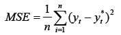
Mean Squared Error (MSE):

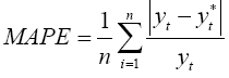
Mean absolute percentage error (Mean Absolute Percentage Error, MAPE):

where n is the number of training examples.

In our case, using the data values shown in Figures 1, 2, 14, and 15 in the calculations, the average absolute error was 2.32%.

The choice of the appropriate forecasting method consists in determining whether this method gives satisfactory forecast errors. In addition to calculating errors, their comparison is carried out in a special Visualizer–"scatter diagram" (Figures 10 and 11). The scatterplot displays the output values for each of the training sample examples, whose X-axis coordinate is the output value in the training sample (reference). Y-axis coordinate is the output value calculated by the trained model in the same example. A straight diagonal line is a reference point (a line of ideal values). The closer the point is to this line, the smaller the model error. The scatter plot is useful when comparing multiple models. It is often enough to look at the diagonal line's spread to determine which model provides the best accuracy on the training set. The work performed by the author on estimating the scatter diagrams of various forecasting models showed that the neural network provides the smallest spread within the boundaries of a given error (Figures 10 and 11).

Conclusion

This paper solves the problem of predicting COVID-19 diseases in Moscow and the Russian Federation using neural networks. This approach is useful when it is necessary to overcome difficulties related to non-stationarity, incompleteness, unknown distribution of data, or when statistical methods are not satisfactory. The forecasting problem is solved using the Deductor Studio analytical platform developed by Base Group Labs (www.basegroup.ru, Russian Federation, city of Ryazan). When solving the problem, we used mechanisms for clearing data from noise and anomalies, ensuring the quality of building a forecast model, and obtaining forecast values for tens of days ahead. The time series forecasting principle was also demonstrated: import, seasonal detection, cleaning, smoothing, building a predictive model, and predicting COVID-19 diseases in Moscow and the Russian Federation using neural technologies for twenty days ahead.

References

1. JunLin, Judy Yong, Shaoyan Guo, Longhan Xia and Gu Xu. “Multi-projection of unequal dimension optimal transport theory for Generative Adversary Networks.” Neural Networks 128(2020): 107-125.

   [Crossref] [Google Scholar]

2. Shi, Yong, Jiabin Liu, Bo Wang and Zhiquan Qi, et al. “Deep learning from label proportions with labeled samples.” Neural Networks 128(2020):73-81.

   [Crossref] [Google Scholar]  

3. Rahman, Abdur, M  Shamim Hossain, Nabil A Alrajeh and Guizani. “B5G and Explainable Deep Learning Assisted Healthcare Vertical at the Edge: COVID-I9 Perspective.” IEEE Network 34(2020):98-105.

   [Crossref] [Google Scholar]

4. Zhao, Amy, Guha Balakrishnan, Fredo Durand and John V Guttag, et al. “Data Augmentation Using Learned Transformations for One-Shot Medical Image Segmentation.” IEEE Comput Soc Conf Comput Vis Pattern Recognit 15(2020):921.

   [Crossref] [Google Scholar]

5. Szegedy, Christian, Wei Liu, Yangqing Jia and Pierre Sermanet, et al. “Going Deeper With Convolutions.”  IEEE Comput Soc Conf Comput Vis Pattern Recognit 1 (2015):1-9.  

   [Google Scholar]

6. Chudzik,  Piotr, Somshubra Majumdar, Francesco Caliva and Bashir Al-Diri, et al. “Exudate segmentation using fully convolutional neural networks and inception modules.” Med Image 2018: Image Process 10574(2018):785-792.

   [Crossref] [Google Scholar]  

7. Zhang, Ruikai, Yali Zheng, Carmen C Y Poon and Dinggang Shen, et al. “Polyp detection during colonoscopy using a regression-based convolutional neural network with a tracker.”Pattern Recognit 83(2018):209-219.

   [Crossref] [Google Scholar]

8. He, Kaiming, Xiangyu Zhang, Shaoqing Ren and Jian Sun. “Deep Residual Learning for Image Recognition.”  IEEE Comput Soc Conf Comput Vis Pattern Recognit 2 (2016):770-778.

   [Google Scholar]

9. Hadsell, Raia, Sumit Chopra and LeCun. “Dimensionality Reduction by Learning an Invariant Mapping.” Conf  Comput Vis Pattern Recognit  5 (2006):1735-1742.

   [Crossref] [Google Scholar]

10. Chollet, Francois. “Xception: Deep Learning With Depthwise Separable Convolutions.” IEEE Conf Comput  Vis Pattern Recognit 5 (2017):1251-1258.

    [Google Scholar]

11. Hossain, Shamim, Ghulam Muhammad and Nadra Guizani. “Explainable AI and Mass Surveillance System-Based Healthcare Framework to Combat COVID-I9 Like Pandemics.” IEEE Network. 34(2020): 126-132.

    [Crossref] [Google Scholar]

12. Wei, Dong, Deng Jia, Richard Socher and Li-Jia Li, et al. “ImageNet: A large-scale hierarchical image database.” IEEE Comput Soc Conf Comput Vis Pattern Recognit 6(2009):248-255.

    [Crossref] [Google Scholar]

13. Valle, Marcos Eduardo and Rodolfo Anibal Lobo. “Quaternion-valued recurrent projection neural networks on unit quaternions.” Theor Comput Sci 843(2020):136-152.

    [Crossref] [Google Scholar]

14. Martí-Ballester, Carmen-Pilar. “Do European renewable energy mutual funds foster the transition to a low-carbon economy?” Renew Energy 143(2019):1299-1309.

    [Crossref] [Google Scholar]

15. Zhang, Sheng, MengYuan Diao, Wenbo Yu and Lei Pei, et al. “Estimation of the reproductive number of novel coronavirus (COVID-19) and the probable outbreak size on the Diamond Princess Cruise ship: A data-driven analysis.” Int J Infect Dis 93(2020):201-204.

    [Crossref] [Google Scholar]

16. Atangana, Abdon. “Fractal-fractional differentiation and integration: Connecting fractal calculus and fractional calculus to predict complex system.” Chaos Solit Fractals 102(2017): 396-406.

    [Crossref] [Google Scholar]

17. Baleanu, Dumitru, Guo-Cheng and Sheng-DaZeng. “Chaos analysis and asymptotic stability of generalized Caputo fractional differential equations.” Chaos Solit Fractals 102(2017):                                        99-105.

    [Crossref] [Google Scholar]

18. Cirillo, Pasquale and Nassim Nicholas Taleb. “Tail risk of contagious diseases.” Nat Phys 16(2020): 606-613.

    [Crossref] [Google Scholar]

19. Driessche, P van den and James Watmough. “Reproduction numbers and sub-threshold endemic equilibria for compartmental models of disease transmission.” Math Biosci 180(2002): 29-48.

    [Crossref] [Google Scholar]

20. Elman, Jeffrey. “Finding Structure in Time.” Cogn Sci 14(1990): 179-211.

    [Crossref] [Google Scholar]

21. Felix, Gers and Schmidhuber. “LSTM recurrent networks learn simple context-free and context-sensitive languages.” IEEE Trans Neural Netw Learn Syst 12(2001): 1333-1340.

    [Crossref] [Google Scholar]

22. Benjamin, Gompertz. “XXIV. On the nature of the function expressive of the law of human mortality, and on a new mode of determining the value of life contingencies. In a letter to Francis Baily, Esq. F. R. S. &c.” Philos Trans Royal Soc 115(1825): 513-583.

    [Crossref] [Google Scholar]

23. Maria, Kiskowski and Gerardo Chowell. “Modeling household and community transmission of Ebola virus disease: Epidemic growth, spatial dynamics and insights for epidemic control.” spatial dynamics and insights for epidemic control, Virulence 7(2016):163-173.

    [Crossref] [Google Scholar]

24. Hyndman, Rob and Anne Koehler. “Another look at measures of forecast accuracy.” P Int J Forecast 22(2006): 679-688.

    [Crossref] [Google Scholar]

25. Philip, Pare E, Ji Liu, Carolyn L Beck and Barrett E Kirwan, et al. “Analysis, Estimation, and Validation of Discrete-Time Epidemic Processes.” IEEE Trans Control Syst Technol  28(2020): 79-93.

    [Crossref] [Google Scholar]

26. Spyros, Makridakis, Evangelos Spiliotis and Vassilios Assimakopoulos. “The M4 Competition: 100,000 time series and 61 forecasting methods.” Int J Forecast  36(2020): 54-74.

    [Crossref] [Google Scholar]