Implementing an Urban Bicycle Highway on Pedestrian Traffic - Finding a Traffic Control Strategy with Optimal Coordination for the City Center of Munich

Arifin Islam¹ and Tasminur Mannan Adnan^2*
*Correspondence: Tasminur Mannan Adnan, Department of Industrial Engineering and Management, University of Oulu, Finland, Tel: 01976067606, Email:

Keywords

Optimal Coordination • Bicycle highway • VISSIM •Traffic control • Traffic efficiency

Introduction

Cycling is gaining popularity all over the world because it’s a fast, energy efficient, healthy and enjoyable mode of transport [1-3]. Interest towards bicycle is increasing eventually as the plans regarding urban and suburban travel behavior and bicycle facilities are designed in a way that both facilitate and encourage use of bicycle for both recreational and day to day commuting travel [3]. Car traffic has always been the focus of research when it comes to urban traffic whereas, a huge number of people living in the urban cities these days are leaning towards bicycles where research is lagging behind [4].

Munich is Germany's third-largest city with a population of around 1.4 million, 500,000 of whom are frequent commuters. In more than 90 percent cases, the total trip length for cyclists is less than 5 km. In Europe, this resulted in 11 percent of all road deaths [5]. The federal government 's target is to raise the share of bicycle travel by 2020 to 15 per cent while rising the rate of fatality by 40% [6] Now-a-days, however, urban development consists of pedestrianoriented patterns, frequently incomplete and unable to anticipate their spatial movement and contact with other transport modes. City designers interested in creating a walking friendly urban area seem to have a greater view of traffic movement [7]. Traffic flow modeling models, however, will routinely test policies and the traffic planning approach. Though most simulation software concentrates on motor vehicle modeling rather than non-motorized [2]. Despite this, there are few microscopic modeling methods available for evaluating traffic planning approaches for both motorized and non-motorized vehicles and taking decisions prior to implementation.

The article is structured in the following way: Section 2 addresses the insights of microscopic traffic flow simulation, calibration and validation of traffic flow simulation, modelling and simulation of bicycle and pedestrian traffic, different microscopic simulation tools, variations of bicycle highway infrastructures, traffic signal control system, and different traffic safety assessment approaches. Section 3 explains the study approach containing research scenario within PTV VISSIM, investigation area, data collection process and necessary steps of base model development. Procedure of model calibration, validation, coordination procedure and safety assessment procedures are discussed in the same section. Chapter 4 presents the alternatives for this article. Five variations of the current situation were developed. The variation between them is discussed in this chapter then. The idea is to compare the alternatives to evaluate them based on selected measures of efficiency. Chapter 5 describes and discusses the outcome from the simulation. Lastly, Section 6, summarizes the main findings and presents the conclusion of the article together with recommendations for future work.

Research Methodology

Overview of microscopic traffic flow simulation

Reuschel in 1950 and Pipes in 1953 first proposed the concept of a model of car following. The following vehicle was believed to want to maintain a total healthy lead time of 1.02 seconds [8]. Car following model is generally considered the foundation of every traffic simulation model being developed. Simulation of follower vehicle actions with the aid of this model [9]. During the late 50s and early 60s the GHR model was a commonly popular model [10]. Chandler et al. produced the initial version of the pattern in 1958 [11]. This model's definition was based on empirical theory, in which vehicle speed is proportional to vehicle acceleration. Subsequent researchers developed various parameter combinations to construct multiple extensions of this [11].

However, the success of this model has diminished due to a large number of contradictory researches.

Gipps car-following concept was created by Gipps in 1981 and its 'collision avoidance' class gained attention. This class model calculates the path to safety and adapts the driving actions of the previous vehicle [10]. This specific approach produces a prediction process very similar to actual traffic decisions and claims that the subsequent driver reacts to minor shifts in the speed of his corresponding car arbitrarily. The model uses two main premises as its basis:

• Driver of the following vehicle is not influenced by the size of the speed variations in case of large distance.

• A limited speed or distance that marks a threshold and as a result the driver of the following car will not respond for short distance.

Models for lane changes consist of two stages. This is the method of lane discovery and the other is the decision to allow lane change. Lane modifications are marked, in most models, as optional (DLC) or compulsory (MLC) [8]. Nagel and Schreckenberg were the first to implement the cellular automation concept for traffic flows [12]. The defined model is a discrete function of space and time. A roadway is composed of cells that mimic the checkerboard or the points in a frame [13]. There are four steps of the model:

• Vehicles that have not reached the highest speed will accelerate by single unit.

• If the velocity of the vehicle (v) is higher than empty cell (m), then the velocity becomes topmost. If the velocity of the vehicle (v) is lesser than empty cells (m), then the velocity changes to v. (v= min [v, m]).

• The velocity of the vehicle could decrease by one unit with the probability p.

• The new position of the vehicle can be decided by the current speed and current position.

Calibration and validation of traffic flow simulation

Calibration and validation are a combination of steps in which model parameters are adjusted to make the simulated model a real-life replica of the situation [14]. Chu suggested a four-step validation technique, which can be used with all models of traffic simulation [15]. Kim and Zhizou carried out separate experiments where they presented analytical solutions, using simplex methods and genetic algorithms. Neither study provided a method for calibrating parameters using VISSIM [16,17]. Hellinga suggested an approach to calibrate that consists of three central phases and eight-part steps [18]. Step 1 consists of tasks that are done before any modeling is begun. Step 2 consists of the primary simulation model validation, based on the real-life scenario details available. Step 3 is a combination of field measurements with simulation process result. The relation takes place against the predefined parameters. If the criteria are met, the simulation model will be accepted. If the criteria are not met, the simulation model won’t be accepted. Changes will then be made to the parameters of the model to meet the requirements. The goal of calibration is to reduce the differences between the simulated model and the MOE’s in field measurements. The process to do that is by adjusting the available parameters [19].

The electronic micro simulation devices provide a number of dynamic parameters to calibrate the model to the conditions in the region. Ultimately, the calibration goal is to define a set of parameter values of the model that better replicates the behavior of local traffic [20]. The simulation models will have specific metrics of efficacy. The choice of this will depend on the purpose of the analysis, the model 's capabilities and the evidence available in the field [20]. Inside the correct efficacy calculation there is a range of output metric, controllable and uncontrollable input parameters [21]. Depending on the chosen efficacy test, different details needed to calibrate and verify the microscopic simulation. Mean and variance of the results from these simulation runs are taken into consideration for assessment. 10 Simulations run primarily considered satisfactory. Probably one of the most challenging aspects of traffic modeling is the development of assessment standards to assess model performance. Subsequently, a statistical confidence level can be established and can be used as appraisal criteria [18].

Modelling and simulation of bicycle traffic

Longitudinal model typically uses concept-based vehicles such as Gazis- Herman-Rothery models, psychophysical concept, and model of safety space. Any modifications are considered, to make it more practical for cycling traffic. Bicyclists select their position by taking into account time to collide with another road user. Figure 1 shows model baseline scenario [22].

Helbing and Molnar developed the idea of the paradigm of social power out of the pedestrian dynamics. In this model three concepts of force are critical. Firstly, a term describing the acceleration in the direction of the desired velocity of motion; secondly, terms showing that a pedestrian maintains a minimum distance from other pedestrians and boundaries; and thirdly, a term modeling attractive impact [23]. Several models for bicycles were proposed based on a model of social force. Li suggested a model on which repulsive force and driving force depend [18]. Liang suggested another concept of collective power, recognizing free movement and congested traffic [24]. Several variations of the standard for modeling road traffic modeling are discussed here:

Thorough simulation of this model by heterogeneous traffic is feasible by designing cell raster. The raster cells are created by taking into account the length and width of the smallest road users. The road users can therefore occupy more than one cell per step in time [22]. Vasic and Ruskin have proposed yet another extension for mixed traffic. The model's idea was to create properly sized cell for bicyclists and car drivers designed by the intersection's roadway geometry. Consequently, the model’s cells overlap as the road users overlap [25].

Modelling and simulation of pedestrian traffic

Pedestrian Modelling is difficult not only due to the enormous number of variables but also due to the situations and environment they face. Simulation offers planners the means to predict the pattern movement of a large number of pedestrians [25]. Space-syntax models were based on the idea of direct perception where pedestrians act by evaluating the graphical properties of the surfaces of footway around them. The decision on the movement is focused on the route which offers better accessibility [26]. STREETS is a simulation model focused on the agents. It as well as mesoscopic spatial scales. It uses a mixture of simple interaction and deterministic way rule-finding, copies the choice of route on microscopic [27].

Dijkstra made a combination of an agent-based approach to simulate pedestrian motion in a shopping mall with a cellular automated approach. The pedestrians were agents that were travelling across a grid of cellular automata. Agents had numerous information, such as their environment, the status of the other agents, their own choices. From these a starting and target position in the area can be selected as the shortest route or the most desirable routes [28]. Fridman and Kaminka were involved in creating a common agent-driven paradigm based on the concepts of based on the concepts of social science theory called Social Comparison theory (SCT). Their agents were reliant on a process that included two actions: comparison and imitation [29]. Models have also been developed where the pedestrians are motivated on the optimum path to reach their destination. The choice of this path is determined by rules relating to ‘social force’. These rules describe the interaction of pedestrians with other pedestrians in a series of crowded contexts [30].

Microscopic simulation tools

Simulation techniques reached a new peak in their demand as researchers became more likely to test out ideas in a controlled atmosphere before playing with them in real life scenario. VISSIM is one of those simulation instruments and PTV created this microscopic traffic simulation [26]. Over the last 15 years, VISSIM has about 7000 licenses issued worldwide [31]. It's capable of simulating traffic in both freeways and urban centers. Particular importance can be given to public transport and multi-modal transport via VISSIM [32]. VISSIM's system architecture primarily includes two modules, the signal state generator and the traffic simulator. VISSIM uses the psychophysical driverbehaviour paradigm developed by Wiedermann. It is used for its consistent conducting behavior in the field [33]. Wiedermann's traffic flow model is based on believing it has four moving states: free moving, trailing, approaching, and braking states. When the car crosses a threshold, the driver changes his condition [34]. PTV VISSIM has an add-on called PTV Viswalk, and IT can be used as part of VISSIM or independently. This can be used in combination with vehicular traffic to represent foot activity [35].

Urban Mobility Simulation (SUMO) is an open source simulation program which uses the model Krauss. It is a pattern-following vehicle, and an evolution of the pattern Gipps. SUMO can simulate critical traffic characteristics, such as free and congested flow [[36]. TRANSIMS is another open source program for simulation of microscopic flows. This is often used at a provincial level for travel planning. TRANSIMS uses various criteria to model human travelers. It has basically four main modules [37].

Cube Dynasim is an event-based program that generates dynamics and stochastic outputs. It has the ability to model a transport system which integrates ITS implementation. It can import data from GIS, CAD, and other datasets. This program for micro simulation also has few configuration methods, depending on the local traffic situation [38]. CORSIM (CORridor Modeling) has achieved attention worldwide as a traffic flow simulation program. It was first adopted by the FHWA [39]. With the implementation of TSIS (Traffic Software Integrated System), it has a user friendly, streamlined interface and framework to run the CORSIM traffic simulation model [40].

Traffic signal control system

The manner in which the traffic signal is managed is categorized into two major types: Isolated traffic signal control and Coordinated traffic signal control [41]. Bang proposed two ways of running the intersections [42]. Isolated traffic signal management can be done in many ways, based on the condition of the intersections and the need for traffic. There are few approaches of isolated traffic signal control: FT (Fixed time signal control), Vehicle actuated control (VA), Self-optimized real time control [41,43]. Coordinated traffic signal control have different approaches: Fixed Time Coordination, Fixed Time Coordination with Traffic Actuated Time Plan Selection, LTA, and Traffic Actuated Time Plan Calculation [41].

Numerous experiments have been conducted to improve traffic signal synchronization. Stamatiadis and Gartner had suggested a bandwidthoriented model of development. It is called the MULTIBAND-96 programme and can provide variable-width progression in traffic networks through arterial roads [44]. Tian has developed a computer program that aims to provide full bandwidth solutions for several randomly generated scenarios of the signal system [8]. Tian and Urbanik have developed a signal synchronization method that is based on a system partition technique. The goal was to maximize the progression spectrum for continuous signals by means of a signalized arterial [45].

Bicycle highway infrastructure

The requirements of a bicycle highway depend on the location and importance of the street in the local and interurban bicycle network (ERA, 2010). Initially, the need for a cyclist is determined by the importance of the link function, the intended level of service and safety features. Dimensions of the space needed for cycling traffic can be derived from a bicyclist’s width and height, and the clearance required for moving them [46]. Table 1 below shows the clearances required to design cycle traffic infrastructure in a safe manner. The measurements required for handling cycle traffic are shown in Figure 2.

Traffic safety assessment

Traffic safety is typically calculated by evaluating previous accident data in terms of incident number and frequency. Often, however, it’s desirable to evaluate the impact of a transition before finally implementing it [35]. Microscopic traffic simulation can be very useful for safety evaluation and prediction purposes, as they allow various designs and traffic parameters to be tested and evaluate the results before applying them in real life [47]. Prior research has found that the scale of traffic, conflict and extreme conflict will forecast accidents and their frequency [48,49]. FHWA developed a variant of software known as the “Surrogate Safety Assessment Model (SSAM). It can perform statistical analysis of vehicle trajectory data from microscopic simulation models [49]. SSAM will have details on five surrogate protection measures: TTC, PET, DR, MaxS, and DeltaS. Several works have shown that SSAM can represent the evaluation of safety from simulated conflicts. One research tried using virtual disagreements to forecast collisions at chosen intersections. The result shows that SSAM received significant associations with real data concerning crashes [50]. Another research analyzed signalized intersections and areas of the freeway to compare the conflicts caused by through VISSIM and SSAM to the observed conflicts in the real life [51].

Overview of Study Approach

Study area

For this research the study area is focused on two major streets in Munich, Leopoldstraße and Ludwigstraße. Combined, the total length of these two streets is approximately 2.5 km from north to south. There are only 10 signalized intersections across the whole network. Figure 3 shows the intersections of the research.

Data collection

The network geometry data, traffic signal control data are provided by the chair of traffic engineering and control, Technical University of Munich (TUM). Traffic demand data were collected by previous students of TUM. All the network geometry data signal control data were generated by Landhauptstadt Munchen. For this analysis PTV VISSIM (Academic License) 2020 (SP 2) [81010] was used to conduct microscopic simulation. That is a complete version of the warrant. Two separate data sets have been used to calibrate and test the model in VISSIM, and the chair of traffic engineering and regulation, TUM provided all the data sets for cars and bicycles.

Research scenario development in PTV VISSIM

The simulated version of the region under investigation was built in few steps at VISSIM. The actions which have been taken and the conclusions made are:

Base data: The geographical state of the region of inquiry must be modified to VISSIM's simulation database. The network environment and simple vehicle modeling objects are all included in the simulation database.

Network coding: The intersections were planned to use the Landeshauptstadt München style. The network roadway was planned by tracing over the OpenStreetMap. In VISSIM, any dynamic intersection can be modeled using the connector and spline. The following Figure 4 shows the structure of network encoding in VISSIM.

This layout uses three types of compositions of the cars. They have a perfect distribution of speed and relative flow of type of vehicle. Table 2 below indicates the vehicle composition for that network.

Model calibration and validation

The following formula is used to derive the number of simulations runs needed.

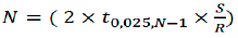
Here the peak value for N is 11.4. As a result, the tuning and testing of the model is known as the rounding up of 12 simulation cycles. Traffic volume is chosen as the MOE was also obtained for the calibration and field measurement data. The seven calibration parameters chosen for this analysis and its values are shown in Table 3 below.

The software validation is performed with a confidence interval of 90%. Root mean square error (RMSE) is used to equate field measurement data collection with simulation performance. Calibration figures are seen in the Table 4 below, based on the vehicles and the level of cycling traffic.

Lastly, calibration results based on pedestrian volume after 12 simulation runs is shown in Table 5 below.

A different new data was used to validate the simulation model. Travel time is used as MOE to validate the model for the simulation. The selected time is the busiest hour in the evening (17:00-18:00). Just like calibration, three different databases were generated to evaluate the vehicles, bicycles and pedestrians travel time data in Table 6 and Table 7.

Traffic signal co-ordination

In this network, two-way coordination is not possible, as the length of the major road from North to South and from South to North is not the same. Coordination will therefore be carried out for vehicles traveling from north to south as it has higher demand for traffic. For this analysis, synchronization was done independently with both the vehicles and the rider. For one-way street, the relationship among speed (v), offset (c) and distance (D) is,

c= D/V

The first move was to measure the offset of the intersections to achieve cohesion with bicycles and vehicles. The pace used for motorcycles were 15 km/h and for vehicles were 40 km/h, which is the same as for simulation. Table 8 displays the offset value used to align the signals for bicycles and vehicles. For each signal category the modified offset value is then added in VISSIM. Improvement was also observed in metrics such as travel time, distance, and number of stops.

Traffic safety assessment

In this research, the Surrogate safety evaluation model (SSAM) was used to evaluate network traffic safety. The criteria used for this analysis are set out below in Table 9. After finalizing the thresholds, the calibrated and validated simulation model was run. The outcome from SSAM is shown in Table 10 below.

Evaluation parameters and settings

In this work the data was collected in VISSIM for a fixed period of 3600 sec. The evaluation settings used for the simulation models are shown in Table 11 below.

Description of Alternatives

Within the validated simulation model, three separate network variants were tested. The differences were made on the basis of bicycle highway width and network synchronization. Increased bicycle highway width was considered for evaluating the bicyclist’s traffic and actions. In the current lane, the width in the bicycle lane varies from 1.5 m to 2.5 m across the network. In the first change the distance of cycling lanes from the present scenario was expanded by 1 m. The second variation was created by increasing the width of the model by 1 m, where the North-South traffic signal is coordinated for bicycles. Finally, another change was suggested by again increasing the width of the cycling lane by 1 m in the simulation model where co-ordination for North-South cars was achieved. The emphasis was on changing road conditions in the path of big traffic flows (Leopoldstr. -Ludwigstr). For the field of research six separate validated models have been developed. The models and their latest headings are listed in Table 12.

Alternative Analysis

Traffic efficiency analysis

In this experiment, we ran the validated model for 12 times for each alternative and picked the peak hour (17:00-18:00). The results were taken from VISSIM as att file (.att), files were imported to excel spreadsheet to analyze the traffic flow efficiency for implementing coordination and increasing bicycle lane width. The network performance is represented through three efficiency indicators, and the indicators are vehicle delay time, number of stops and travel time. The research outcome was presented through Box and Whisker Plot diagram. The lines extended both up and down outside the rectangle are known as Whiskers, for example shown in the Figure 5 below. The difference between the first quartile and the third quartile is known as interquartile range (IQR). The models and their representative colour are shown in Table 13.

Delay time

Vehicle delay time is calculated by deducting the theoretical travel time from the actual VISSIM travel time. Figure 5 shows Cars' wait time for the alternatives from North-South direction. Traffic synchronization for cars from the North-South route, in Figure 5, had a major effect on the vehicle wait time for cars as it decreased for C3 and W3. The delay time increased where priority was given to bicycle lanes either by coordination or by widening lanes, as in C2, W1 and W2. Figure 6 below indicates the delay period for the cars coming from the South-North route.

The delay time in C3 was lowest and the delay time in C2 decreased by 18% and in C3 by 29%. Car delay time increased by 11% in W2 and the highest in W2. However, in Figure 7, considering the delay time for bicycles moving from North to South, it can be seen that delay time in all alternatives has decreased. W2 had the largest drop in wait time by 29%.

Lane widening and traffic signal coordination for bicycles decreases delay time for both cases. Bicycles going from South to North, Figure 8 reveals that the delay period in W1 was reduced by 7%. The delay time for C3 remains close but in all the other situations a significant improvement in delay time was observed. Widening bicycle lane assisted in reducing delay time in W1.

Number of stops

Another metric for measuring traffic performance is the number of exits in the alternatives. Figure 9 shows the number of cars stops in north to south direction. The number of stops fell by almost 50 percent in both C3 and W3, and there was signal synchronization for cars in the north-south direction, which explains the fall. C2 had a 6 per cent drop, W1 had a 12 per cent decline in number of exits. Whereas the number of stops remained essentially the same for W2. C2 had a 6 per cent drop, W1 had a 12 per cent decline in number of exits. Whereas the number of stops remained essentially the same for W2. The number of stops decreased for W1, W2 and W3 for the cars going from South to North, as seen in Figure 10 below. For these three options saw the cycling lanes extended. Number of stops decreased by 26% and 11% respectively for C2 and C3. For these three options saw the cycling lanes extended. Number of stops decreased by 26% and 11% respectively for C2 and C3.

However, for bicycles going from North-South, the number of stops for both C2 and W2 shown in Figure 11 decreased by 28%. The number of stops declined by 12% for W1. Widening cycling lanes helped the bicyclist to make the line shorter. As a result, several bicyclists may ride side by side resulting in the number of stops declining. On the contrary, the number of stops in C2, W2 and W3 which is shown in Figure 12 below for bicycles moving from South-North increased. The highest increase was 28% for W3. W2 and C2 had an increase in the number of stops by respectively 25% and 4% whereas the number of stops decreased for C3 by 8% and for W1 by 5%.

Travel time

Vehicle travel time is yet another measure of performance. Figure 13 shows the typical travel time for cars going North to South. The overall travel time was lowered by 18% in C3. The average travel time in W1 rose by 4% and in W2 by 7%. Car synchronization in north to south direction has played a significant role in rising average travel time in C3. The Figure 14 below shows the travel time of automobiles moving in the South to North direction. In C2 and C3, travel time was reduced by 8% and 2% respectively. The average travel time increased by 14% in all other alternatives where the highest was in W2.

With the alternate W3 from Figure 15 below, the total travel time with bicycles going from North-South remains exactly the same. We can observe a decrease in average travel time for C2, W1 and W2. There is a significant decline in W2 where the total travel time has declined by 7%. A 6% decrease was also reported for C2 and a 4% decrease in total travel time for W1.

The above Figure 16 shows the average travel time for bicycles traveling from the direction of South-North. The only alternative where the average bicycle travel time has decreased compared to the current scenario is W1, where it has decreased by 3%. The average journey time for the other alternatives increased. The highest increase was 18 per cent in the case of W2 which also includes outliers.

Review of key events in animation

It can be noted from the 3D animation that teamwork has played a major role in improving the traffic performance. The length of the queue was shorter, as most cars went across the green wave. This benefited the right turning cars, because other cars could not use the lanes, so they earned more time to make the turn. Widening lanes for cyclists helped them cross the road more easily. It also helped the right turning cars as they needed to wait less time for the cyclists to cross, so they received a bigger share of the green light. On a whole, coordination provided better traffic efficiency for bicycles then just widening the lane.

Traffic safety assessment

In this study the validated model for current peak hour (17:00-18:00) was considered for the review of traffic safety. VISSIM results were taken output as file format in trj file (.trj). The file was then imported into SSAM to assess the safety of the models in traffic. To evaluate network health, two performance metrics were selected. The Time to Collision (TTC) and Post markers encroachment time (PET).

Safety assessment overview

Figure 17 represents the TTC Value of the network area alternative models. It can be observed that the time to collide from the current model, C1, decreased in C2 and C3. Whereas in W1, W2 and W3 the TTC value increased by 7%, 10% and 6% respectively. Bicycle highway system growth helped improve road safety as bikers obtained more space to ride. The post-intrusion time (PET) of the alternate models can be measured from Figure 18 below, where the post-intrusion time from the existing model C1 decreased in C2 and C3. Whereas the PET value in W1, W2 and W3 rose by 3%, 5% and 1% respectively. Bicycle highway infrastructure development helped drive traffic safety, as bikers gained more space to travel side by side. The integration of road synchronization for cars and enhancement of the cycling network has resulted in the strongest PET increase for W2.

Pedestrian traffic safety assessment

The highest average TTC value in alternative C3 was achieved in Figure 19, where it improved by 31 per cent. It remained almost the same for W3, whereas all other alternatives observed an increase. But TTC's value is less than the overall value of a network. It involves greater risk to pedestrians than other shareholders in the traffic. Also, the PET value involving pedestrians is lower than the overall performance of the network that can be observed from Figure 20. Compared to the current model the value again remained almost the same for W3. PET changes were found in all other models which included outliers as well.

Interaction between pedestrian and Bicycle

Seeing that the pedestrian footpath and the cycling lane are adjacent to each other, contact poses certain safety concerns. The Table 14 below shows the potential relationship of alternative models and the form of collisions between them. For model W1, the highest TTC value was reached followed by W2. For W1, W2 and W3 the PET values were also higher than for C1, C2 and C3. Growing lane width for cyclists demonstrates the increase in post-intrusion period. In simulation model, the number of collisions between pedestrians and cyclists was smaller for C2 and W2, where synchronization for bicycle traffic is done in the direction of north to south. For C3 and W3, the number of collisions is higher and are both modeling models where vehicle traffic synchronization is implemented. It indicates planning here has an effect on the number of collisions.

Visual assessment of road safety

VISSIM 3D animation was used to visually illustrate the safety factors of the simulation models. The estimation indicates the most likely crash happened at the intersections of road users. Right turning vehicles waiting to cross the pedestrian produced some circumstances of collision nearby. Similar situations also occurred between bicycles and cars, but there was comparatively less frequency of such situations. Lane changing also forced cars to be in less safe than usual situations.

Conclusion

The aim of this research was to define a strategy for traffic control that will provide the highest efficiency for different participants in the traffic. A particular attention was granted to pedestrians in evaluating the effect of bicycle highway pedestrian. The findings of the alternative study demonstrated change in the efficiency of bicycle traffic flow mainly in the models where bicycle teamwork was implemented. Bicycle lane widening also helped increase the traffic efficiency but was not as successful as teamwork. Bicycle traffic management resulted in a decrease in travel time for cyclists by up to 7 per cent. The number of stops for organizing cycling traffic even reduced significantly. Widening cycling lane helped in facilitating right-turning traffic flow. The model's road safety evaluation indicates that both teamwork and road lane widening have substantial impacts. All the popularity of TTC and PET improved as the cycling lanes widened. The pedestrian-bike experience indicates that the probability of collision between them is greater than that of other actors in the traffic. Versions with synchronization for road traffic have saw fewer pedestrian-bike accidents than other proposed models. While this research contains literature reviews in the field of microscopic traffic flow, simulation model testing and evaluation, traffic management techniques, and approaches for achieving traffic signal synchronization. In addition, literature research was conducted on the simulation and modeling of the development of bicycle traffic and bicycle infrastructure, as well as methods for assessing traffic safety of simulation models

For further improvement, inclusion of parking lot and public transport could be considered as it will impact on simulation result. Similar study could also be conducted by widening bicycle lane might also have an impact in the overall performance in the network. Moreover, other traffic control strategies can be considered for further analysis in the future.

Though VISSIM was used as the simulation tool for this study, other microsimulation tools can be applied to evaluate which simulation tool gives less relative error and better flexibility for calibration and validation of the simulation model [52-55].

References

1. Menghini, G, Carrasco N, Schüssler N and Axhausen KW. “Route choice of cyclists in Zurich.” Transportation Research Part A: Policy and Practice 44 (2010): 754-765.  
2. Milakis, Dimitris and Konstantinos Athanasopoulos. “What about people in cycle network planning? Applying participative multicriteria GIS analysis in the case of the Athens metropolitan cycle network.” Journal of Transport Geography 35 (2014): 120-129.  
3. Li, Zhibin, Wei Wang, Pan Liu and David R Ragland. “Physical environments influencing bicyclists’ perception of comfort on separated and on-street bicycle facilities.” Transportation Research Part D: Transport and Environment 17 (2012): 256-261.   
4. Ma, Xiaoliang and Ding Luo. “Modeling cyclist acceleration process for bicycle traffic simulation using naturalistic data.” Transportation Research Part F: Traffic Psychology and Behaviour 40 (2016):130-144.   
5. Huemer, Anja Katharina. “Motivating and deterring factors for two common traffic-rule violations of cyclists in Germany.” Transportation Research Part F: Traffic Psychology and Behaviour 54(2018): 223-235.   
6. https://www.ncbi.nlm.nih.gov/pmc/articles/PMC3821406/
7. Kitazawa, K and Batty M. “Pedestrian behaviour modeling.” (2004).   
8. Toledo, Tomer. “Driving behaviour: models and challenges.” Transport Reviews 27(2007): 65-84.
9. Mitroi, Ionuț-Sorin, Ana-Maria CIOBÎCĂ and Mihaela POPA. “Car-following models comparison between models used by VISSIM and AIMSUN.” UPB Sci Bull (2016).
10. Brackstone, Mark Mike McDonald. “Car-following: a historical review.” Transportation Research Part F: Traffic Psychology and Behaviour  2(1999): 181-196.
11. Vasconcelos, Luis, Luís Neto, Sílvia Santos and Ana Bastos Silva,  et al. “Calibration of the Gipps car-following model using trajectory data.” Transportation Research Procedia 3 (2014): 952-961.
12. Schreckenberg, Michael and Kai Nagel. “A cellular automaton model for freeway traffic.” J Phys I France  2 (1992): 2221.
13. Ding, D. “Modeling and simulation of highway traffic using a cellular automaton approach.” (2011).  
14. Park, Byungkyu and JD Schneeberger. “Microscopic simulation model calibration and validation: case study of VISSIM simulation model for a coordinated actuated signal system.” Transportation Research Record 1856 (2003): 185-192. 
15. Chu, Lianyu, Henry X Liu and Will Recker. “Using microscopic simulation to evaluate potential intelligent transportation system strategies under nonrecurrent congestion.” Transportation Research Record 1886 (2004): 76-84. 
16. Kim, Kyu-Ok and LR Rilett. “Simplex-based calibration of traffic microsimulation models with intelligent transportation systems data.” Transportation Research Record 1855 (2003): 80-89. 
17. Zhizhou, Wu, Sun Jian and Yang Xiaoguang. “Calibration of VISSIM for shanghai expressway using genetic algorithm.” In Proceedings of the Winter Simulation Conference (2005).
18. Hellinga, BR. “Requirements for the calibration of traffic simulation models.” Proceedings of the Canadian Society for Civil Engineering 4 (1998): 211-222.  
19. https://www.nhtsa.gov/sites/nhtsa.dot.gov/files/documents/florida_fy2017_ar.pdf
20. file:///C:/Users/srishti/Downloads/dot_41797_DS1.pdf
21. Twaddle, Heather, Tobias Schendzielorz and Oliver Fakler. “Bicycles in urban areas: Review of existing methods for modeling behavior.” Transportation Research Record 2434 (2014): 140-146.
22. Helbing, Dirk and Peter Molnar. “Social force model for pedestrian dynamics.” Physical review E 51(1995): 4282.  
23. Liang, Xiao, Baohua, MAO and Qi XU. “Psychological-physical force model for bicycle dynamics.” Journal of Transportation Systems Engineering and Information Technology 12 (2012): 91-97. 
24. Yaldi, Gusri and Wen Long Yue. “The use of CUBE Dynasim and aaSIDRA in analyzing a signalized intersection.” In 29th Australian Transport Research Forum, Canberra ACT 2601 (2006).
25. Hillier, B, Penn A, Hanson J and Grajewski, T, et al. “Natural movement: or, configuration and attraction in urban pedestrian movement.” Environment and Planning B: Planning and Design 20 (1993): 29-66.  
26. Haklay, Mordechai, David O'Sullivan, Mark Thurstain-Goodwin and Thorsten Schelhorn. “So go downtown.”: simulating pedestrian movement in town centres. Environment and Planning B: Planning and Design 28 (2001): 343-359. 
27. Dijkstra, J, Timmermans HJ and Jessurun AJ. “A multi-agent cellular automata system for visualising simulated pedestrian activity.” Springer (2001): 29-36.
28. Fridman, Natalie and Kaminka, Gal A. “Comparing human and synthetic group behaviors: A model based on social psychology.” (2009).  
29. Helbing, Dirk, Péter Molnár, Illés J Farkas and Kai Bolay.  “Self-organizing pedestrian movement.” Environment and Planning B: Planning and Design 28 (2001): 361-383.  
30. Fellendorf, Martin and Peter Vortisch. “Microscopic traffic flow simulator VISSIM.” Fundamentals of Traffic Simulation (2010): 63-93.  
31. Papageorgiou, Georgios Nathaniel. “Towards a microscopic simulation model for traffic management: a computer-based approach.” IFAC Proceedings Volumes 39 (2006): 403-411.   
32. Maciejewski, M. (2010). “A comparison of microscopic traffic flow simulation systems for an urban area.” Transport Problems 5: 27-38.  
33. Ptv Ag, Karlsruhe. “Ptv Vissim User Manual.” (2020).  
34. Axelsson, Eva and Therese Wilson. “Microscopic simulation as an evaluation tool for the road safety of vulnerable road users.” Digitala Vetenskapliga Arkivet (2016).
35. Krajzewicz, D., Hertkorn, G., Rössel, C., & Wagner, P. (2002). SUMO (Simulation of Urban Mobility)-an open-source traffic simulation. In Proceedings of the 4th middle East Symposium on Simulation and Modelling (MESM20002) (pp. 183-187).  
36. Lee, Kwang Sub, Jin Ki Eom and Dae-seop Moon. “Applications of transims in transportation: A literature review.” Procedia Computer Science 32 (2014): 769-773.
37. Yang, ZhenYu and Zhijun Ding. “Actuated green wave control for grid-like network traffic signal coordination.” IEEE International Conference on Systems, Man, and Cybernetics (2016): 000953-000958.
38. Chien, Steven I.-Jy, Kyriacos C Mouskos and Shoaib M Chowdhury. “Generating driver population for the microscopic simulation model (CORSIM).” Simulation 76 (2001): 40-45.
39. Owen, LE, Zhang Y, Rao L and McHale G. “Traffic flow simulation using CORSIM.” Winter Simulation Conference Proceedings 2 (2000):1143-1147.
40. Al-Mudhaffar, Azhar. “Impacts of traffic signal control strategies.” (Doctoral dissertation, KTH) (2006).
41. Bång, KL and Nilsson LE. “Optimal control of isolated traffic signals.”IFAC Proceedings Volumes, 9(1976): 173-184.
42. Young William, Amir Sobhani, Michael G Lenné and Majid Sarvi. “Simulation of safety: A review of the state of the art in road safety simulation modeling.” Accident Analysis & Prevention 66 (2014): 89-103.
43. Stamatiadis, Chronis and Nathan H Gartner. “MULTIBAND-96: a program for variable-bandwidth progression optimization of multiarterial traffic networks.” Transportation Research Record 1554 (1996): 9-17.   
44. Tian, Zong, Mangal, Varun and Liu Hongchao. “Effectiveness of lead–lag phasing on progression bandwidth.” Transportation Research Record 2080 (2008): 22-27.
45. Forschungsgesellschaft für Strassen, Verkehrswesen (Germany) Arbeitsgruppe Verkehrsführung, & Verkehrssicherheit. Hinweise zur mikroskopischen Verkehrsflusssimulation: Grundlagen und Anwendung FGSV Verlag 388 (2006).  
46. “Recommendations for cycle traffic installations.” (2010).
47. Manual, HC. “Transportation Research Board of the National Academies.” (2010).
48. https://rosap.ntl.bts.gov/view/dot/35896
49. Huang, Fei, Pan Liu, Hao Yu and Wei Wang. “Identifying if VISSIM simulation model and SSAM provide reasonable estimates for field measured traffic conflicts at signalized intersections.” Accident Analysis & Prevention 50 (2013): 1014-1024.  
50. Fan, Rong, Hao Yu, Pan Liu and Wei Wang. “Using VISSIM simulation model and Surrogate Safety Assessment Model for estimating field measured traffic conflicts at freeway merge areas.” IET Intelligent Transport Systems 7 (2013): 68-77.  
51. Sadid, H.  “Integration of Public Transport Prioritization and Bicycle Signal Coordination in Traffic Signal Control,“ Master Thesis in Transportation System (TUM).” (2018).  
52. Aziz, Md Tariq. “Comparing two different traffic simulation environments for simulating urban bicycle highway traffic – the case of SUMO and PTV VISSIM,.” MASTER’S THESIS.” Technische Universität München (2018).   
53. Turner, Alasdair and Alan Penn. “Encoding natural movement as an agent-based system: an investigation into human pedestrian behaviour in the built environment.” Environ Plann B Plann Des 29 (2002): 473-490.
54. Willis, Alexandra, Nathalia Gjersoe, Catriona Havard and, Jon Kerridge, et al. “Human movement behaviour in urban spaces: Implications for the design and modelling of effective pedestrian environments.” Environ Plann B Plann Des 31 (2004): 805-828.
55. Tian, Zong and Thomas Urbanik. “System partition technique to improve signal coordination and traffic progression.” J Transp Eng 133 (2007): 119-128.