Comparative Study of Operating Modes for Low-power Wireless Sensor Networks in Vibration-based Machine Condition Monitoring

David Alexander Ells^*, Christopher Mechefske and Yongjun Lai
^*Correspondence: David Alexander Ells, Department of Mechanical and Materials Engineering, Smith Engineering, Queen’s University, Kingston, ON, K7L 3N6, Canada, Tel: +16135336535, Email: ,

Keywords

Wireless sensor network • Capacitive MEMS accelerometer • Machine condition monitoring • Vibration analysis • Data processing

Introduction

Sensor Networks (SNs) and Wireless Sensor Networks (WSNs) can be used to measure conditions such as temperature, pressure, and vibrations to monitor systems or environments [1,2]. More specifically, these networks can be used for machine condition monitoring by performing vibration analysis [3-5]. Machine condition monitoring can offer several benefits including improved performance, reduced operating costs, and enhanced safety. The most common methods of vibration analysis for machine condition monitoring include time domain and frequency domain analysis [6-8].

For the purpose of machine condition monitoring, WSNs can offer several advantages over traditional SNs. These advantages include ease of deployment, greater flexibility, better scalability, and reduced cost [4]. However, WSNs present new challenges with respect to managing energy consumption and battery life, and data processing and management [1,2].

Considerable research has been done to address these challenges with power consumption and battery life [9,10]. Solutions include optimizing the hardware, software, configuration, and routing of the WSN for low-power operation. The hardware can be optimized by using specifically designed low-power controllers, sensors, and antennas. Software-based solutions include optimizing data collection, processing, and transmission. More specific data reduction solutions include local data aggregation, compression, and prediction [9]. Since transmitting data consumes more energy than processing, it has often been reported that data processing and reduction performed on the end node can reduce the net power consumption [1,2,11].

With advancements in Micro-Electro-Mechanical Systems (MEMS), battery technology, and data processing methods, WSNs are becoming more effective, and these challenges can be overcome. The objective of this work was to develop a WSN that can effectively perform vibration-based machine condition monitoring with low power consumption by incorporating these recent advancements. A WSN end node is presented, that is based on a capacitive MEMS accelerometer and an integrated microcontroller. The necessary software was developed to perform time and frequency analysis, and a new data reduction method is presented that reduces the frequency spectrum while preserving the important data. The hardware and software of the WSN end node was then tested experimentally, and its energy consumption was compared for different operating modes with the objective of determining the best data processing method for low-power operation.

Materials and Methods

End node hardware

The WSN end node is based on the ATmega256RFR2 Microcontroller (MCU) and a KX132 capacitive MEMS accelerometer. An image of the end node prototype can be seen in Figure 1. The ATmega256RFR2 is a highperformance, low-power AVR 8-Bit microcontroller from Atmel, with 256 KB flash memory, 32 KB internal SRAM memory, 8 KB EEPROM, and integrated 2.4 GHz radio transceiver. The KX132 is a three-axis accelerometer with a selectable measurement range from ± 2 g to ± 16 g and is capable of sampling at a rate of 25600 Hz. The microcontroller and accelerometer communicate through the SPI interface (Figure 1).

Data processing method and development

The end node was programmed to collect 1024 acceleration samples at a rate of 1600 Hz. The 16-bit samples were converted to acceleration in g, stored as 4-byte decimals, and the mean was removed. The mean removal involved calculating the average of the samples and subtracting it from each sample in-place. The size of the converted acceleration data was 4096 bytes total.

Time domain analysis

Calculating the max acceleration and the RMS parameters is a relatively low-memory and low-complexity process. The peak amplitude is simply the largest absolute sample of acceleration, and the RMS is the square root of the mean square of the set of samples. For a discrete set of numbers, the RMS is calculated as follows [7]

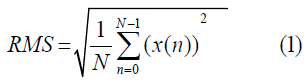
Table 1 shows the program memory, data memory, and compute time for processing 1024 samples on the end node. The size of the peak amplitude and RMS results were 4 bytes each (Table 1).

Frequency domain analysis

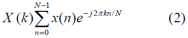
Converting the acceleration over time to the frequency domain can be done with several different transforms. The most commonly used algorithms are based on the Fourier Transform, called Fast Fourier Transforms (FFTs). These algorithms compute the Discrete Fourier Transform (DFT) to process finite-length, discrete-time signals with fewer operations. The DFT is defined as follows, where X(k) is the computed frequency, x(n) is the input signal, N is the number of samples, and j is the imaginary unit [7,8].

Typically, FFTs reduce the number of operations needed to compute the DFT by taking advantage of the symmetry of the expression. While the DFT computes the sum directly and has a complexity of O(N²), FFTs reduce the complexity to O(N log N). There are many different FFT types and permutations that can be implemented to reduce complexity and improve performance for the specific use case.

FFTs can use a recursive or iterative structure. The difference between these structures can affect the complexity, compute speed, and what other permutations may be incorporated in the algorithm. Depending on the size of the dataset, FFTs can use different radices. Common implementations include radix-2, radix-3, radix-4, and mixed-radix FFTs. The radix can affect the complexity, the memory needed, and the compute speed of the algorithm. As well, FFTs can use a Decimation In Time (DIT) or Decimation In Frequency (DIF) structure, however there is no inherent difference in performance between the two.

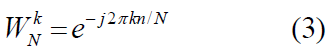
A commonly implemented strategy is to precompute the twiddle factors. In the context of DFTs, twiddle factors are the complex exponential constants, defined as follows.

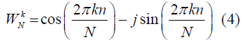
The twiddle factors can also be expressed using cosine and sine functions [7]. Where, the cosine term represents the real part, and the sine term represents the imaginary part.

By precomputing and storing these constants, the algorithm reduces the number of redundant computations, trading the use of additional memory for reduced compute time. These permutations cater to specific applications and balance trade-offs between complexity, memory usage, flexibility, and compute speed.

Several different FFT algorithms were written and tested on the WSN end node. Table 2 below, compares the program memory, data memory, and compute time processing 1024 samples for each algorithm. All FFTs used the same predefined complex type and macros for the complex operations. Of those tested, the FFT with the fastest compute time was a recursive radix-2 decimation-in-time FFT algorithm with precomputed twiddle factors. The FFT used 1690 bytes in program memory and took 0.6350 seconds to complete. The size of the resulting frequency spectrum data is 4 bytes per magnitude, and 2 bytes per frequency (Table 2).

There are many other methods that can be used to reduce the compute time of FFTs. These include optimizing the data type, optimizing the memory access and allocation, reducing the number of operations, and optimizing the operations and macros. Several different methods were tested in the development of the FFT algorithms. Table 3 presents a comparison of complex type and operation method used. By implementing a complex type structure rather than the compiler complex type, and macros for the complex operations, the compute time was reduced by 12.65 percent for the fastest FFT algorithm (Table 3).

Frequency spectrum data reduction

The objective of the data reduction method was to reduce the frequency spectrum to the fewest data points necessary while preserving the relevant information. The process was separated into two steps, correcting the magnitude of the frequency spectrum, and defining the peaks to be selected.

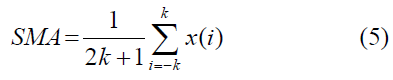
The purpose of the correction step was to normalize the spectrum and emphasize peaks based on local prominence. The process calculated the simple moving average, of a user configurable window size, and divided the frequency amplitude by this average. The simple moving average is defined as follows, where k is the offset, and 2k + 1 is the total size of the average window. The greater the window size is, the smoother the average and the better the correction result, but the greater the compute time.

A predetermined number of peaks were then defined as the greatest local maximum inside a window of configurable size. The amplitude and frequency of the peaks were then saved. Table 4 compares the memory and compute time of the selective data processing method for different numbers of selected peaks with a moving average offset of 10 and a local maximum offset of 2. The size of the reduced data was 384, 192, 96, and 48 bytes for 64, 32, 16, and 8 selected peaks respectively (Table 4).

Vibration testing setup

To test the WSN end node and data processing method, it was mounted to a LabWorks ET-139 permanent magnet vibration shaker, as seen in Figure 2. The shaker was powered and controlled by an Agilent 33220A arbitrary waveform generator and a LabWorks PA-141 linear power amplifier. A calibrated PCB model 288D01 impedance head was mounted to the same plate as the end node and served as a reference accelerometer. The data collected and processed by both the WSN end node and the PCB impedance head was monitored and saved on a computer (Figure 2).

Results and Discussion

Data processing results

To evaluate the performance of the WSN end node, the shaker was programmed to generate discrete sine waveform vibrations at 100, 200, 300, 400, 500, and 600 Hz. Figure 3 compares the acceleration samples of PCB impedance head and the WSN end node for the 100, 200, and 300 Hz shaker tests. The plots show the magnitude of acceleration in g vs. time in seconds (Figure 3, Tables 5 and 6).

The magnitudes of both the max acceleration and RMS results for the end node are significantly less than those measured on the PCB impedance head. This discrepancy may be the result of several factors including less secure packaging of the accelerometer, greater damping from additional components, and lower sensitivity of the MEMS accelerometer.

Figure 4 shows the frequency spectrum of the WSN end node measurements plotted for each of the 100, 200, 300, 400, 500, and 600 Hz shaker tests. The plots show the magnitude of acceleration in g vs. frequency in hertz. In each case the characteristic frequency is accurately measured and clearly shown (Figure 4).

Table 7 compares the peak frequency of the FFT results for the PCB impedance head and the WSN end node (Table 7).

While the WSN end node can accurately measure and clearly show the characteristic frequency of the vibration, the magnitude of the acceleration is significantly less than what was measured on the PCB impedance head. This discrepancy in magnitude is reflected in the FFT results and is highlighted by the difference in peak frequency magnitude.

To evaluate the selective data processing method, the shaker was programmed to generate a multi-sine-on-random waveform. The signal was a sum of sine waves at 30, 60, 100, 120, 200, 240, 300, and 400 Hz of different amplitudes and some randomly generated number.

The vibration shaker was programmed to generate the signal with the Agilent 33220A arbitrary waveform generator. Both the PCB impedance head and the WSN end node collected and processed the vibration data separately. Table 8 compares the max acceleration and RMS result for the PCB impedance head and the WSN end node (Table 8).

Figures 5 and 6 compare the frequency spectra for the data collected by the PCB impedance head and the WSN end node for the multi-sine-on-random waveform. The memory needed to store the frequency spectrum data is 3072 bytes (Figures 5 and 6).

The results for the WSN end node show the same decrease in magnitude with increase in frequency as seen in the peak acceleration and RMS results. While both spectrums show the same characteristic frequency responses, the end node results are significantly lower. For example, the peak frequency magnitude at 400 Hz in the WSN end node results is 68.8 percent less than in the PCB impedance head results.

The end node then performed the selective data processing method. Figure 7 shows the frequency spectrum collected and processed by the WSN end node after the spectrum correction process was performed. Most notably the lower magnitude peaks at 200, 300, and 400 Hz are enhanced relative to the rest of the spectrum (Figure 7).

The program then performed the peak selection process. To demonstrate the data reduction method for different numbers of peaks, the peak selection process was performed for 64, 32, 16, and 8 selected peaks. The memory needed to store the reduced data was 384, 192, 96, and 48 bytes respectively. Figure 8 compares these results. It can be seen that all 8 characteristic sine waves are preserved in the data reduced to 8 peaks. Depending on the machinery or system being monitored, and the complexity of the vibration signal, the number of selected peaks can be configured (Figure 8).

To assess the performance of the data reduction method, it was tested and compared to a basic data reduction method. Both methods were tested using the same dataset of 1024 samples and configured to select 8 representative peaks for analysis. The basic method selected the 8 largest numbers by magnitude. The results, presented in Table 9, show the trade-off between memory, compute time, and effectiveness. While the corrective data selection method needed more memory and compute time, it successfully selected all 8 characteristic sine waves (Table 9).

Energy consumption results

The energy consumption of the end node was then measured and compared for different operating modes. The results are shown in Table 10 below. Operating mode (a) involved collecting and transmitting the raw acceleration data. Vibration data was collected, converted to acceleration (in g) that was stored as decimals, at 4 bytes per sample or 4096 bytes total, and transmitted to the gateway. Operating mode (b) involved collecting, processing the data, and transmitting the processed data packet. After collection, the vibration data was processed locally to determine the max acceleration, RMS parameter, and frequency spectrum, 2056 bytes total, and transmitted to the gateway. Operating mode (c) involved collecting, processing, correcting and selectively reducing the data and transmitting the reduced data. After time and frequency analysis was processed locally, the frequency spectrum was corrected and selectively reduced to 8 peaks, resulting in a reduced data packet of 56 bytes total. Operating mode (d) involved collecting, processing, and selectively reducing the data and transmitting the reduced data. The last operating mode (e) involved collecting and processing the vibration data, checking thresholds, and not sending any data if the thresholds were not met. This method, presented in [11], is intended to save energy by not transmitting any data unless a predetermined threshold is met. For testing purposes, no data was sent (Table 10).

Every strategy that involved processing data locally to reduce the size of the data packet, consumed more energy than transmitting the raw data. Processing and transmitting the data packet reduced by 49.8 percent consumed 31.0 percent more energy. Processing and selectively reducing the data packet by 98.6 percent consumed 8.8 to 21.4 percent more energy, depending on the data reduction method. And processing the data, comparing it to thresholds, and not sending any data consumed 7.4 percent more energy. These results likely differ from other reports because of the specific hardware and software that was implemented. Specifically, the low-power MCU that was used. Transmitting data was relatively low-power, and data processing was relatively slow, consuming more energy than expected.

Conclusion

In this work, a novel WSN end node was presented for machine condition monitoring. The necessary software to perform vibration analysis was developed, and a data reduction method was proposed to reduce the frequency spectrum and the size of the data packet. The performance of the WSN end node was tested experimentally, and its energy consumption was compared for different operating modes.

Tests showed that the WSN end node was capable of collecting and processing vibration data successfully. While the results were not as accurate as the reference accelerometer, the capacitive MEMS accelerometer was not expected to have the same level of sensitivity. These results can still be effectively monitored for trends and use hardware-specific thresholds for machine condition monitoring.

The proposed data reduction method was shown to reduce the frequency spectrum more effectively than past methods. The magnitude correction step successfully emphasized peaks in the frequency spectrum based on local prominence, resulting in less of the characteristic responses being accidentally discarded. As well, the peak selection step allowed for more configurability in how the characteristic responses were selected. However, the improvement in effectiveness came at the cost of additional compute time and power consumption.

Results for the comparison of energy consumption for different operating modes did not match expectations or other reports. Every mode that processed the vibration data locally to reduce the packet size consumed more energy than transmitting the raw data. While the data packet was reduced by 98.6 percent, results showed that processing and reducing the data locally consumed 8.8 to 21.4 percent more energy than transmitting the raw data. It can be concluded that, for the WSN end node presented, transmitting raw vibration data is a better strategy for low-power operations than processing the data locally.

Acknowledgment

None.

Conflict of Interest

None.

References

1. Yang, Kun. “Wireless sensor networks.” (2014).

Google Scholar, Crossref

2. Akyildiz, F. and M. C. Vuran. “Wireless Sensor Networks.” Wiley (2010).

Crossref

3. V. C. Gungor. “Industrial wireless sensor networks: Applications, protocols, and standards.” CRC Press/Taylor & Francis (2013).

Google Scholar, Crossref

4. Hou, Liqun and Neil W. Bergmann. "Novel industrial wireless sensor networks for machine condition monitoring and fault diagnosis." IEEE Trans Instrum Meas 61 (2012): 2787-2798.

Google Scholar, Crossref, Indexed at

5. Neuzil, Jan, Ondrej Kreibich and Radislav Smid. "A distributed fault detection system based on IWSN for machine condition monitoring." IEEE Trans Instrum Meas 10 (2013): 1118-1123.

Google Scholar, Crossref, Indexed at

6. Scheffer, Cornelius and Paresh Girdhar. “Practical machinery vibration analysis and predictive maintenance.” Elsevier (2004).

Google Scholar

7. Ahmed, Hosameldin and Asoke K. Nandi. “Condition monitoring with vibration signals: Compressive sampling and learning algorithms for rotating machines.” JWS (2020).

Google Scholar, Crossref

8. Jain, Prashant H. and Santosh P. Bhosle. "Analysis on vibration signal analysis techniques used in diagnosis of faults in rotating machinery." Int J Mech Prod Eng Res Develop 10 (2020): 3377-3396.

Google Scholar, Indexed at

9. Anastasi, Giuseppe, Marco Conti, Mario Di Francesco and Andrea Passarella. "Energy conservation in wireless sensor networks: A survey." Ad Hoc Networks 7 (2009): 537-568.

Google Scholar, Crossref, Indexed at

10. Rault, Tifenn, Abdelmadjid Bouabdallah and Yacine Challal. "Energy efficiency in wireless sensor networks: A top-down survey." Comput Netw 67 (2014): 104-122.

Google Scholar, Crossref, Indexed at

11. Bergmann, Neil W. and Li-Qun Hou. "Energy efficient machine condition monitoring using wireless sensor networks." icWC (2014): 285-290.

Google Scholar, Crossref, Indexed at