A Spatial-Nonparametric Approach for Prediction of Claim Frequency in Motor Car Insurance

Kipngetich Gideon^*
*Correspondence: Kipngetich Gideon, Department of Pure and Applied Sciences, Pan African University, Nairobi, Kenya, Tel: 0708366735, Email:

Keywords

Nonparametric • SAR • Smoothing Spline • Claims • CIC • Spatial

Abbreviations

CIC: Cooperative Insurance Company

DP: Dirichlet Process

GB2: Generalized Beta of the Second Kind

PLS: Penalized Least Square

SAR: Spatial Autoregressive

LL: Local Linear

Introduction

Insurance has a fundamental role in providing financial protection and offering a transfer risk in exchange for an insurance premium. Therefore, estimation of the right premium for the policyholders is the noblest task in the insurance business. Insurance companies provide insurance to policyholders, and in turn, the policyholders have to pay insurance premiums through the agreed time (periodically). Due to competition in the market, charging a fair premium according to the policyholder’s expected loss is profitable for the insurer. The company will attract more customers and boost customer relationships with the insurer. The amount of premiums paid by the policyholders is determined from estimates of their expected claim frequencies and the claims’ severity. Setting precise and reliable estimates of claims frequencies has extreme importance.

Recent studies on spatial modeling have been rapidly applied in many fields; epidemiology, public health, and the Insurance sector. Different models commonly employed to fit current claims data and predict claim frequencies are Poisson regression models, generalized linear models, Credibility models, Bayesian Models. However, from the available literature, these models appear to be relatively inflexible. Essentially all models are wrong, but some are useful, which is true when the process being modeled is either not well understood, or the necessary data are not available [1]; the same problem of choosing the model is experienced in the modeling of the claims, Although the generalized linear models provide accurate and fast analysis of insurance data, they fall short because they are defined based on the assumptions, and an incorrect model assumption can cause model misspecification leading to erroneous results. Nonparametric models are deemed to minimize the shortcoming of these standard parametric models since fewer assumptions are made for the model, therefore, suitable for modeling insurance data which are nonlinear, nonparametric models perform better than generalized linear models (GLMs) [2], the only observable problems with modeling using Nonparametric models are the interpretation of some of their curves. When modeling claims and risks, we need to determine their behavior and spatial dependence, and spatial heterogeneity of the data so that the insurer can determine which areas are associated with a higher riskier when determining premiums amount to be paid.

[3] propose a Bayesian nonparametric approach for prediction of claims, here they found out that the model performs better compared to nonparametric GLMs in that it can capture the nonlinear random effects present in the data, [4] also propose a flexible nonparametric loss model for prediction of the claims, they found out that having flexible multivariate model may allow actuaries to estimate the dependence between different risk classes and different lines of business and this topic need to be explored further, and introduce the idea of using nonparametric data mining approach to modeling of the claims and prediction of risk, here the approach classify risk and predict claim size based on data. This study’s research idea was to build based on the study by [5,6] where they introduce a nonparametric spatial regression model for prediction. This study’s primary objective is to construct a spatial nonparametric estimator for the prediction of insurance claims. Therefore, this study’s main contribution was to investigate the estimator’s performance in the situation of additional covariates in the model and incorporate the aspect of spatial dependence in constructing a nonparametric estimator for the prediction of insurance claim frequencies.

The main difference between this research and [6, 7] are as follows: (1) estimate a nonparametric spatial model where estimation of the unknown trend g (·) is based on smoothing spline (2) Rather than assuming that spatial correlation takes a particular form (as in SAR), spatial correlation and spatial heterogeneity are considered simultaneously with second order stationarity (3) the estimators’ asymptotic properties under mild conditions.

Methods and Materials

In this section, we propose methods of estimating a claim frequency model for prediction. The basic claim frequency model is introduced, stressing the need to introduce a new method of estimating a more flexible claim model where the basic model restriction is relaxed. The spatial effects are incorporated to complete the proposed model.

Claim Model

Claim model is used a generalized linear model in modelling aggregate claims in non-life insurance [8]. This aggregate claim model can be improved by adding a more attractive feature on the way the fit is. Defined the following terms

1. Claim severity is the total claims divided by the number of claims (average size per claim)

2. Claim frequency is the number of claims divided by the duration (average number of claims per unit time)

Most traditional claim models have assumed that the claim follows a Poisson process with a rate λ; on the other hand, claim severities follow a continuous model, and gamma distribution has been extensively used. The aggregate claim model is given by

S_t= X₁ + X+…+ X_Yi

Where S_t is the aggregate claim amount of a given trading yearn t, Y_i is random number that denotes the number of claims in a year t, X_i with i = 1,2,…Y_i is the amount of i^th claim realized in the year t. Some of the important assumptions as defined in the model equation (1) include

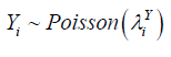
Y_i ~ Poisson λ for some0 < ƛ < ∞ are iid ∀i

Y_i and X_i are independent ∀i

X_i are iid ∀i Traditionally in insurance practice, the claim frequency has been modelled following Poisson distribution and X_i has the form of the loss distribution, i.e., separate gamma distribution for the claim severity [9]. Modeling the frequency of claims, let Y_i denotes the number of claims involving i policies at time t, then the total expected number of claims Y is expressed as

m is the total number of observed policies, Y_i is mostly assumed to follow discrete distribution of which Poisson distribution has been commonly used in many models. Y_i depends on covariates such as the region where the policy was taken, age, sex, type of vehicle, number of claims per policy, years of policy ownership, insured cases number for a user and average claim size, then

Where mean is given by

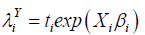
X_i is covariate vector for i^th observation and is assumed to have linear relationship with Y_i, t_i denotes the exposure time of policyholder i and β_i denotes a vector of unknown regression parameters.

The assumptions on X_i and Y_i are mispecifications, and if the data appear to be nonlinear, it will create a substantial modeling bias. Therefore, a nonparametric method is proposed; the main aim of this nonparametric technique is to relax highly restrictive regression function [10].

Model Estimation

The study proposes a nonparametric regression model to predict the number of claims Y_i, i = 1,….n observed in region J in order to relax restrictive assumption on the distribution of number of claims and X_i covariates vector for the i^th claim. Since claims in each region, J has nonlinear relation with the covariates X_i' s . The nonparametric form of the model is given by the general form [11, 12].

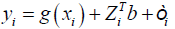
G (.) is unknown nonparametric function used to model fixed effects, Z_i^Tb

and ε_i for random unobserved effects. Since the form of  Z_i^Tb = R_i   for R_i  is

 Let  I = (1,...,1)^Tand  n = (n₁,..., n_N  )^Tbe two N  dimensional vectors. We make assumption about the spatial model as

          (2)

Where, i =(i₁,… ,i_N) in Ʌn will be referred to as site, R_i cater for the spatial effects (Random effects) and the cardinality of Ʌ_n is [13].

Modeling spatial data as a finite realization of a vector stochastic process indexed by _{R = (R ,…,R )} R = (R_i … R_n)^T follow joint Gaussian distribution here E(R_i) = 0, σ² = var(R_i) and ∀_i ∈Λ_n 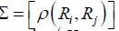correlation coefficient matrix that need to be estimated. For the vector 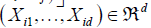Y_i∈ R and

g (·), the unknown function g (·), need to be estimated for 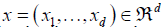, the response variable Y_i is claim frequency and X_i is six dimensional vector consisting of the following explanatory variables: gender, claim amount, age of the policyholder, gender, vehicle age, model of the vehicle and age category of the policyholder.

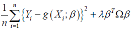
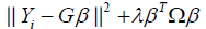
Estimating g(x) at some point x∈R^d for X_i in the neighborhood of x, g(X_i) can be estimated by using smoothing spline [14]. The estimator ( ) ^ g (⋅)of g (⋅) is the minimizer of

                (3)

Which can be represented as

where G∈R^n×n is basis matrix defined as

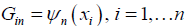
Where 1, n ψ …ψ are the truncated power basis functions with knots at x₁,… x_n which is evaluated at the data values

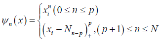
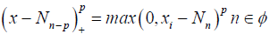where p is compact interval. p is the degree of the spline and 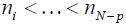are fixed points or knots in φ .

Ω∈R^n×n is the penalty matrix defined as

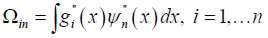
Given the optimal coefficients ^{^}β minimizing (3), the smoothing spline estimate at x is therefore defined as

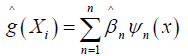
The term affects shrinking components of estimation ^{^}β towards zero. The parameter ƛ ≥ 0 is the smoothing parameter.

Each computed coefficient corresponds to a particular basis function ψ_n. the term β^TΩ β in (3) imparts more shrinkage on the coefficients that correspond to wigglier functions ψ_n(x) . Hence, as we increase ƛ, we are shrinking away the wiggler basis functions. Similar, to least squares regression, the coefficients minimizing (3) is

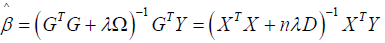
The smoothing spline can be seen as linear smoother, therefore we represent as

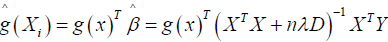                  (5)

which is linear combination of the points Y_i, i = 1, …n and X is a design matrix with entries x_i for i = 1, …,n, Y, Y is a vector of the response variables, D is a diagonal matrix with p +1 zeros on the diagonal followed by N ones and nλD is a penalty term ƛ is estimated as

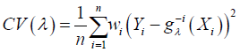               (6)

Where is the smoothing spline estimator fitted from the data less the i^th data Since Σ in model equation (2) is unknown, we assume that R_i, i = 1,2,…, n is 2^nd˗ order stationary and isotopic process. Then let C(h) and γ (h) be covariogram and variogram respectively, where the distance between two locations is given by h [15,13] Then

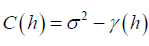
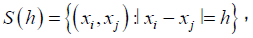
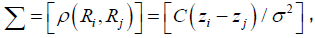while z_i and z_j are the spatial locations associated with error values R_i and R_j, so it is appropriate to estimate γ (h) for Σ [16,17]

          (7)

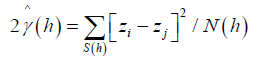
N (h) is a number of distinct pairs in S (h). The characteristics of the estimator (7) can be estimated using Integrated square [18], given by

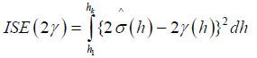
Where h₁ and h_k are the lags [16]. Therefore, since has been estimated then

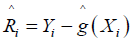
Since R(z_i), the error at location z_i, is unobserved, this quantity must be estimated as well. We use the iterative procedure [13]:

Obtain by means of (4). Then put

Obtain

Using (5), obtain

and go to 2. Step 3 then produces and

Repeat this process to obtain and

The study selects ϵ > 0, i.e., ϵ = 0.001 and the procedure ends when

As proposed by [5, 6] R2 is used to assess the performance of predictors, given by

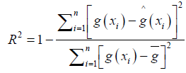
g̅

Where g̅ is the mean of g(x_i), i=1,…,n.

Theoretical properties of Estimator

To obtain asymptotic results, we impose the following assumptions on model (2)

A1. The random field {X_i,i ϵ Ʌ_n} is strictly stationary.

A2. The function g (·) is twice differentiable and its matrix of second derivatives at x denoted by g"(∙) is continuous at all x ϵ.

A3. The process R_i, i = 1,2,…, n is 2^nd order stationary and isotopic, further ∃ a ϵ > 0 such that 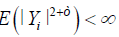for i = 1,2, … , n

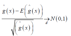
Theorem 1: Asymptotic Normality

In addition to A1-A3, suppose that are iid with mean 0 and variance σ²I_n then, for any xi ϵ and for some constant C > 0 then

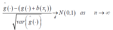           (8)

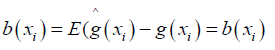
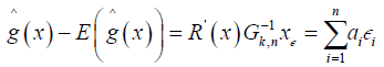
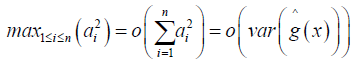
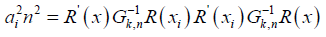
Where b (x_i) is asymptotic bias [19], given by

Proof of Theorem 1: For m > 1, S (m,t) is a set of spline functions with knots of step functions with jumps at the knots and for m ≥ 2

Expressing function in S (m,t) in terms of B-splines for fixed m and t, let

Where [t_i-m, …, t_i]f denote the m^th – order divide difference of the function f and t_i = t_{min(max(i,0),ko +1)} for any i = 1- M, …, k we assume that

And where 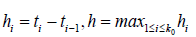and M > 0 (predetermined constant) this assumption ensure that M^-1 < k₀h < M , which is necessary for numerical assumptions

Let D_n (x) be an empirical distribution function of with a positive continuous density d(x) this implies 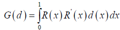Then

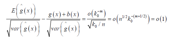
Thus equation (8) follows if

we have

Where 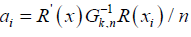the required Lindeberg-Feller conditions, it suffices to verify that

we also have

Finally, equation (8) follows from the assumption that k0 / n → ∞ hence the prove.

Theorem 2

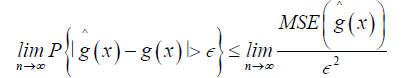
Consistency: From theorem 1, we can establish the asymptotic consistency where for ϵ > 0

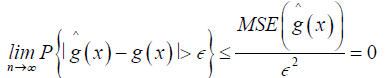                   (9)

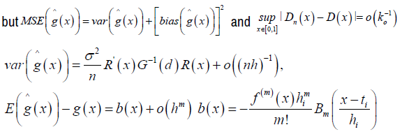
Where B_o (x) =1,

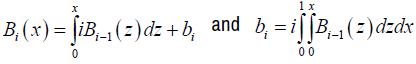is the i^th Bernoulli number [20]. From equation (9)

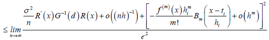       (10)

As n→ ∞ the numerator terms in RHS of equation (10) collapse to zero therefore

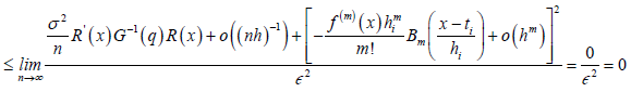
Hence the prove of equation (9), therefore we conclude that the estimator is consistent to the true function g(x) of equation model (2).

Data Description

The study used data from Cooperative Insurance Company’s motor thirdparty liability insurance for 2018 and 2019. 6500 policies are included in the data. The following policy information was used: the area where the policy was purchased, policyholder age, gender, vehicle type, number of claims, years of policy ownership, claim amount, and insured cases number. Age is categorized into three categorize; Old (50 > years), young (<25 years) and Middle age (25-50) (Table 1).

Table 1 shows that there is a very large number of observations has no claims in claims dataset where the maximum number of claims made in a region were 4 in an observation. The histogram in (Figure 1) of the observed claims shows that the distribution of claims is skewed to the right, therefore there is element of over-dispersion in the data due to large number of zeros.

Simulation Results

This section describes the simulation process and the results of the method proposed in this research. This study proposed a model proposed by [6,13] given by

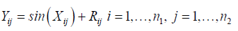
Where Y_ij are the observations and X_ij is a saptial process which represents the explanatory variables and R_ij is the term for spatial effects? The semivariogram is estimated as

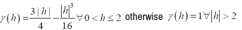
Where h is the distance between 2 locations z_i and z_j in 2-dimensional space X_ij is a spatial process and follows a mean 0 and second order stationary gaussian process, for this reason we use spectral method to simulate X_ij given by

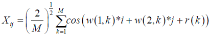
w(i, k ) k =1,…,M are iid normally distributed and are independent of r(k) iid uniform random variables on [―π, π] as n → ∞, X_ij converges to a gaussian ergodic process [17]. The matrix of random errors

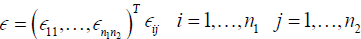are iid normally distributed.

We set the basis function as

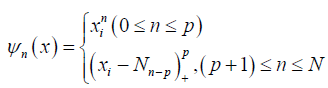
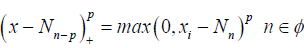where Φ is compact interval. p is the degree of the spline and n_i < …<n_N-p are fixed knots in Φ To measure performance of estimators, we use R² given by

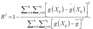
where g̅ is the sample mean of g(Xi), i = 1, .., n. The closer R² to 1 the better the performance of the estimators. Comparing the performance of the proposed method with the other immediate existing methods such as nonparametric spatial models with general correlation structures a method proposed by [13] where estimation was based on kernel estimation and the nonparametric spatial autoregressive (SAR) method under which R = ρ WR + ϵ proposed by [6].

Table 2 shows the simulation results of R² values from 100 simulations. We can see that R² for the proposed method is the largest and closer to 1; this demonstrates the superior performance of the proposed method.

Analysis for claims data

The study considers the claims data from CIC insurance observed in different parts of 42 counties of Kenya to illustrate the performance of the proposed method procedures, which exclude the 5 counties from the northern part of the country since the information regarding the 5 counties was not available. Since we are mainly interested in predicting the claims frequency, the study considers a set of 6500 observations data observed from 42 counties. Let Y_i denote the claim frequency, and Xi = (X₁, …., X₆) T be a vector which consists of the following explanatory variables: gender, claim amount, age of the policyholder, gender, vehicle age, model of the vehicle and age category of the policyholder. By using the following model where, we can predict claim frequencies.

Where Y(z_i):i = 1, … , n is the observations (claims) in region z_i associated with independent variable X(zi) in region z_i, R(z_i) is the unobserved error in region z_i and g(.) is the estimated function. The observations are from a random process observed over a countable collection of spatial regions (county). The data at a particular location typically represent the entire region. Claims data resides on an irregular lattice, with each site representing an entire county [22]. Using R² to measure the performance of the predictor, R2 is defined as

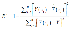
From the analysis of the data, the results were presented in the following table (3).

From table 3 the R² of LL (local linear method) without unobserved random correlation errors is 0.7125 the proposed method outperforms LL model with R² value of 0.9484. In presence of spatial effects, as the iterations increase the performance of the proposed method is significantly better than that of the LL. It is observed that R² increases very little in columns 5 and 6.

Discussion

The construction of the estimator aims at obtaining a robust method for the prediction of claims frequencies. The proposed method adopts a nonparametric approach where smooth function estimated using smoothing spline accounts for the fixed effects.

A random effect (spatial error) was added to the model to improve the prediction. From the simulation study, two methods; Nonparametric model with SAR error [6] and Nonparametric model with the correlated error, which uses kernel in the estimation [13] were compared to the proposed method. The results showed that the proposed method has a significantly better prediction performance of 0.9962 (99.62 efficiencies) compared to the two methods, which have R² values 0.9587(95.87% efficiency) and 0.9691(96.91% efficiency), respectively. The proposed method was applied to the Cooperative Insurance Company (CIC) claims data-set. The findings showed that the proposed model is more efficient with R2 of 0.9544, which is closer to 1 (100% efficiency) in predicting the claims frequencies compared to the Local Linear fitted model with no account for spatial effects with R2 of 0.7125(71.25% efficiency). The proposed method could now be applied to other classes of insurance claims due to its efficiency and capability to capture the nonlinear effects and spatial effects characterized by claims data.

Conclusion

The idea of deriving an appropriate estimator in predicting frequency claims in the insurance industry has gained more interest in finance and statistical research. Many researchers heavily rely on parametric estimators; however, the insurance datasets have some aspect of non-linearity. Hence, researchers in statistics are developing nonparametric estimators with spatial error to improve the prediction based on existing parametric models. The study constructed a spatial nonparametric estimator for predicting claim frequencies in motor insurance, and the theoretical properties of the estimators were derived. The study established the theoretical properties of the proposed estimators under mild conditions. The study found that the proposed nonparametric spatial method is more efficient from the simulation results and application of the method to claims data with 6500 observations than the Local Linear fitting models and nonparametric model with Spatial Autoregressive error in the prediction of claims frequencies. Therefore, based on the results, the proposed method can be applied in predicting claims frequencies due to its efficiency and capability to capture the nonlinear effects characterized by claims data.

Limitations & Recommendations for Further Studies

Some additional exogenous variables may influence claim frequency. For example, the environmental factors among other institutional factors. It is important to investigate how each of the factors affects the output variable. Thus, a more robust spatial estimator for studying the relationship between an output variable and input variables may be constructed in subsequent studies using the proposed method. The data set used in the study involves policies for cars taken by the CIC insurance company. However, in the insurance, there are also policies for life insurance. Hence, further studies should consider the use of other claims data sets (i.e., for life and property claims data sets) in demonstrating the applications of the constructed estimator and also consider developing a more efficient nonparametric package to map Lattice observations under this proposed method.

Limitations of the Study

The data used in the study is Lattice data (without a coordinate system); therefore, there was difficulty in classifying the claims to a specific area in the region (County).

Acknowledgments

I would like to thank the Pan African University for their support and enabling environment also the CIC company for accepting to share their claims datasets which aid in accomplishing the objective of the study.

Conflicts of Interest

The authors declare no conflict of interest.

Appendix

The CIC insurance company did not provide URL link for accessing the data instead they provide an excel sheet containing the data.

References

1. Dursun A. "A comparison of the nonparametric regression models using smoothing spline and kernel regression." WASET 36 (2007): 253-257.
2. Barrow, David L, Chui C, Smith P, and Ward J. "Unicity of best mean approximation by second order splines with variable knots." Math Comput 32, no. 144 (1978): 1131-1143.
3. Box, George EP, and Draper N. Empirical model-building and response surfaces. New York: Wiley 424 (1987).
4. Cressie, Noel. Statistics for spatial data. John Wiley & Sons (2015).
5. Doupe, Patrick, Faghmous J, and Basu S. "Machine learning for health services researchers." Value Health. 22 (2019): 808-815.
6. Dudley, Claire. "Bayesian analysis of an aggregate claim model using various loss distributions." Eidenburg: Disertasi Heriot-Watt University (2006).
7. Fellingham, Gilbert W, and Kottas A. "Parametric and nonparametric bayesian methods to model health insurance claims costs." University of California at Santa Cruz, Department of Applied Math and Statistics Technical Reports (2007).
8. Fellingham, Gilbert W, Kottas A, and Hartman B. "Bayesian nonparametric predictive modeling of group health claims." Insur Math Econ 60 (2015): 1-10.
9. Green, Peter J, and Bernard W. Silverman. “Nonparametric regression and generalized linear models: a roughness penalty approach”. Crc Press, 1993.
10. Hall, Peter, and Opsomer J. "Theory for penalised spline regression." Biometrika 92 (2005): 105-118.
11. Hall, Peter, Kay JW, and Titterington DM. "Asymptotically optimal difference-based estimation of variance in nonparametric regression." Biometrika 77 (1990): 521-528.
12. Hong, Liang, and Ryan Martin. "A flexible Bayesian nonparametric model for predicting future insurance claims." N Am Actuar J 21 (2017): 228-241.
13. Huang, Chunfeng, Hsing T, and Cressie N. "Nonparametric estimation of the variogram and its spectrum." Biometrika 98 (2011): 775-789.
14. Karcher, Peter, and Wang Y. "Generalized nonparametric mixed effects models." J Comput Graph Stat 10 (2001): 641-655.
15. Kašćelan, Vladimir, Kašćelan L, and Buric M. "A nonparametric data mining approach for risk prediction in car insurance: a case study from the Montenegrin market." Econ Res-Ekon Istraz 29 (2016): 545-558.
16. Laslett, Geoffrey M. "Kriging and splines: an empirical comparison of their predictive performance in some applications." JASA 89 (1994): 391-400.
17. Li, Yinghua, Qin Y, and Li Y. "Empirical likelihood for nonparametric regression models with spatial autoregressive errors." J Korean Stat Soc (2020): 1-32.
18. Overmars, Koning D, and Veldkamp A. "Spatial autocorrelation in multi-scale land use models." Ecol Modell 164 (2003): 257-270.
19. Rice, John A, and Colin O. Wu. "Nonparametric mixed effects models for unequally sampled noisy curves." Biometrics 57 (2001): 253-259.
20. Shen, Xiaotong, Wolfe DA, and Zhou S. "Local asymptotics for regression splines and confidence regions." Ann Stat 26 (1998): 1760-1782.
21. Wahba, Grace. “Spline models for observational data”. SIAM 1990.
22. Wang, Hongxia, Wang J, and Huang B. "Prediction for spatio-temporal models with autoregression in errors." J Nonparametr Stat 24 (2012): 217-244.