The topological features of the Valent integrable case on the Lie algebra e(3)

Ghorbanali Haghighatdoost^*
*Correspondence: Ghorbanali Haghighatdoost, Department of Mathematics, Azarbaijan Shahid Madani University, Tabriz, Iran, Email:

Keywords

Integrable hamiltonian system • Bifurcation diagram • Iso-energy surface • Non-degenerate critical points

Introduction

The topological classification theory of integrable Hamiltonian systems had been developed in the papers of fomenko. This approach was new to integrable systems and it was proposed by fomenko and developed further by fomenko, zieschang, bolsinov, oshemkov and some others. Many authors are interested the integrable Hamiltonian systems on some Lie groups. Well-known integrable cases are found on the Lie algebras e (3), so (4) and so (3, 1). All of them have topologically analyzed by Fomenko’s School, namely the Sokolov integrable cases on so (4) which introduced by V.V.Sokolov have investigated by the first author and his colleagues.

The Hamiltonian systems one (3) with a nontrivial additional integral which is polynomial of degree one or two are completely described (such as the Euler, Lagrange, Kovalevskaya, Clebsch, Steklov, Sokolov cases). Up to now, only two families of Hamiltonian systems one (3) admitting an integral of degree three are topologically studied, namely the families of Goryachev-Chaplygin top and the Dullin- Matveev case [1].

Case Study

Selivanova provided an existence proof for some integrable models on two dimensional manifolds with a cubic first integral [2]. However, the explicit form of these models hung on the solution of a nonlinear third order ordinary differential equation which could not be obtained.

Valent showed an appropriate choice of coordinates which gives the explicit local form for the full family of integrable systems. Many of these systems are globally defined and contain some special cases of the integrable systems due to goryachev, chaplygin, dullinmatveev, tsiganov and yehia which some of them was studied before (dullin-matveev case studied recently by moskvin. In this paper, we study a new case which has been obtained by valent [3].

In this system, there exist three parameters α, β and ρ that two of them are free creating some complexities in computations all over this problem such that more results will be showed for zero value of the parameter α [4].

Preliminary

In this section, we recall some necessary facts about integrable hamiltonian systems. A Hamiltonian system one (3) relative to the Lie-poisson bracket has the form:

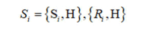
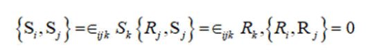
which the bracket is defined in terms of the natural coordinates S₁, S₂, S₃, R₁, R₂, R₃ on the e(3):

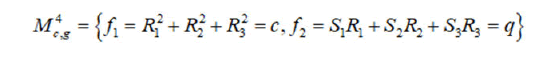
The Liouville integrability of a Hamiltonian system one(3) is equivalent to the existence of one additional integral which is functionally independent of the Hamiltonian H on common fourdimensional level surfaces of the two invariants of the Lie algebra e(3):

That means an integrable Hamiltonian system with the integrals H and K are in involution with respect to the Lie-Poisson bracket on M⁴.

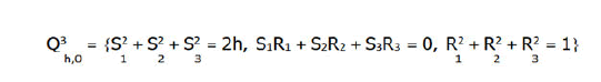
The iso-energy surfaces are 3-dimensional manifolds of the form

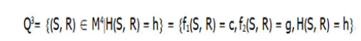
Some linear transformation preserves the bracket 2, then we shall assume in what follows that c=1 and also, we content ourselves straight away with h such that, first, Q³ is compact and, second, dH dH=0 everywhere on Q.

Assume that the following condition holds at the point ξ0 ∈ M⁴:

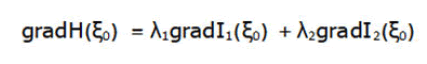
Then the quadratic form defined by the Hessian of the function H=H|M at the point €0 is the restriction of the following matrix form to the tangent space T€ M⁴

G=d²H-λ₁d²I1-λ₂d2I2

Results

First, calculating bracket {H, K} for H and K in system 1, we see that it is zero on all level surfaces f₂=g, that is, H and K are in involution on all 4-manifolds M⁴ [5]. Therefore without considering any additional assumptions on the system 1, we can study this case globally on M_{¹, g}.

Proposition 2: The set of all critical points of rank zero of the mapping f₂ × H for the integrable Hamiltonian system with Hamiltonian H_{1, g} restricted on the orbit M⁴ is equal to:

€_1,2=(gR₁, 0, gR₃, R₁, 0, R₃) s.t

Obviously when α=0, €_1,2=(0, 0, g, 0, 0, 1) and when g²=-2β we also have a degenerate critical point (0, 0) [6]. This immediately implies that for each critical point of rank zero R₂=0 or α=0. Equating to zero the other components and considering all possible variants, we obtain the above result. After that, it is easy to check that sgradK also vanishes at the points indicated [7].

The bifurcation diagram Σ is the image of the set of critical points of the momentum mapping f₂ H in the plane R₂ (g, h). We investigate the bifurcation diagram for system in two cases: α =0 and α =0 [8]. In the first case, when α =0 and for the diff erent values of β. When α=0 we have one type of the diagram: Two parabolas without intersection.

The diagrams are the values of the critical points set in proposition.

The topology of the iso-energy surfaces

One of our results in this paper is caculation of the topology of the iso-energy surfaces Q³ for different values of g and h and the parameters α , ρ , β (Figure 1).

Theorem 3: The critical points of proposition 2 are non-degenerate and the critical points corresponding to the critical value zero are degenerate, so that the energy integral H is almost everywhere a Morse function on M_⁴.

When α=0, β<0, €1 is a saddle point and €₂ is a minimum point, when α=0, β >= 0 or when α0, ξ₁ is a minimum point and €₂ is a saddle point.

Each connected component of an iso-energy surface Q³ for these cases has the following topological types: S³, RP³ correspond to different domains in the plane R² (g, h).

For all the points (g, h) that belong to the same connected component of the set R₂ (g, h), the topological type of Q³ is same, because H is a proper map. Hence, in this special bifurcation diagram, it is enough to find the topology of Q³ i.e the iso-energy surface for g=0. By using lemma1, we calculated G|TM^₄ at every critical point.

Due to space limitation, the calculations are not shown here. Hence for each h, g between two parabola the iso-energy surface Q³ is diffeomorphic to S³ as a level surface of a Morse function in the neighbourhood of a local minimum.

Consider now Q³ for the top of parabolas.

Qh,g is preserved with a smooth substitution

Then Q³ is represented with this surface as:

This surface is already diffeomorphic to RP³, so that the energy surfaces Q³ for the top of parabola is diffeomorphic to RP³.

We can also prove the last and main result of this theorem simply by using the Smale’s theorem

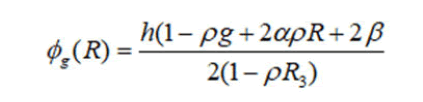
Studying the topological type of Q³ with helping the Smale’s theorem turns out that the topology of iso-energy surfaces and their bifurcations under varying the energy level h is completely determined by the function ϕg(R) which called the reduced potential and obtained with intersecting two surfaces f₂=g and function ϕg(R) which called the reduced potential and obtained with intersecting two surfaces f₂=g and H=h under the projection π:(S, R).

R as some subset of the Poisson sphere S₂, R₃ (R₁, R₂, R₃). For under considering case, we have

In the first case when α=0, ϕg(R) is linear and it’s corresponding Reeb graph can be easily found. In the second case when α=0, ϕg (R) is a function of R₁ and R₃, therefore, we draw the level line of ϕg(R) that is projected to the (R₃, R₁)-plane on the disk R₂+R₂ ≤ In the both cases (α=0, α0) we have one possibility for the corresponding Reeb graph of the graph of the function.

According to the suggested algorithm by Bolsinov and Fomenko using Smale’s theorem, the topological type of the 3-manifold Q³ for all cases are indicated (Figure 2).

The type of critical points of rank zero

To calculate the Fomenko invariants (molecules), we need to investigate the bifurcation of the Liouville tori. For this purpose, we consider the non-degenerate points of rank zero of the integrable system with two degrees of freedom and obtain the type of these points. A critical point of rank zero will be a non-degenerate singular point of the momentum mapping F if the subalgebra K (H, F) is a Cartan subalgebra of sp (4, R). We can see that the subalgebra K (H, F) is generated by the linear operators AH and AF which obtained from linearization of the vector fields sgradH and sgradK at this point.

A commutative subalgebra of sp (4, R) will be cartan if and only if it has dimension 2 and contains a linear operator λAH+μAF with distinct eigenvalues.

There exist four types of non-degenerate points of rank zero with classifying these points on the basis of eigenvalues of this linear operator:

Center-center: four purely imaginary eigenvalues iA, iB, -iA, iB;

Center-saddle: two real and two imaginary eigenvalues iA,B,-iA,-B;

Saddle-saddle: Four real eigenvalues A, -A, B, -B;

Focus-focus: Four complex eigenvalues A+iB, A -iB, -A+iB, -A-iB.

For the integrable system when α =0, the non-degenerate critical points of rank zero have the following types

when β>0, 1<ρ<1/3, €^₂: Center-center, €^₁: Focus-focus;

when β>0, 0<ρ<1/3

If g²<-4βρ/3ρ-1

Then €^₂: Center-center, €^₁: Center-center;

If g²<-4βρ/3ρ-1

Then €₂: Center-center, €₁: Focus-focus;

When β<0, 1/3 <ρ<1,

If g²>-4βρ/3ρ-1

Then €₂: Center-center; €₁: Focus-focus

If -4βρ/1+3ρ<g²<-4βρ/3ρ-1

Then €₂: Center-center, €₁: Center-center;

If g²<-4βρ then €₂: Focus-focus, €₁: Center-center;

In addition, when g²=-2β we also have a degenerate critical point (0, 0).

We shall calculate the operators AH and AF at the critical points.

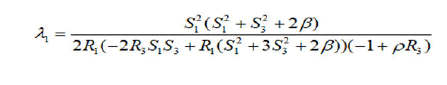
where πij is the Poisson tensor of e(3) anλ₁d, λ₂ are obtained from gradH|€=λ₁gradf₁|€+λ₂gradf₂|€

Considering that discriminant of the characteristic polynomial of the operator AH-AF|TM4 (€_1,2)

We obtain four different purely imaginary eigenvalues when D>0 and four different complex values when D<0. Then all above cases are easily resulted.

Critical points of rank one and the bifurcation diagram for α=0

The critical points are the points at which the skew gradients of the Hamiltonian and integral F are depend. For finding the critical points of rank one we calculate the skew gradients of H and F then set all minors of the matrix sgradH/sgradF equal to zero and restrict the obtained set to M4 (Figure 3).

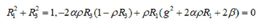
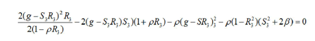
The critical point of rank one of system 1 for α=0 is the following family on R₆: S₂R₁-S₁R₂=0, 2S₂(S₂R₃-S₃R₃)(ρR₃+1)-ρR₂(S₂ +2β)=0;

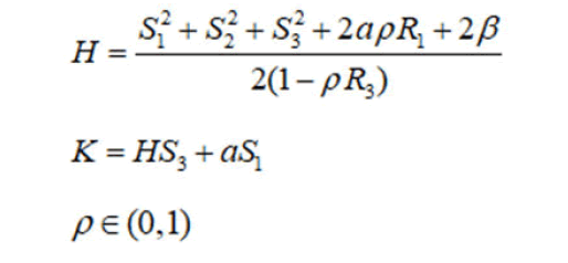
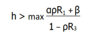
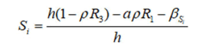
Theorem 6: The bifurcation diagram of the moment map in the valent case for α=0 is obtained from the following equations on M⁴.

k=hS₃+ S₃+2β-2h (1+ρR₃)=0

Proposition 7: α=0 all critical circles of the curves in the bifurcation diagram are non-degenerate means the integral K has no saddle critical circles.

Conclusion

We see from the minors of the matrix sgradH/sgradF that if R=0 then R=0 or S=0. If R=0, the zero rank critical points are founded.

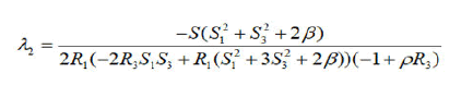
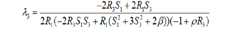
Then we consider now R₂=S₂=0, S₁₀. On this critical points set we consider the matrix G=GH-λ₁G1-λ₂G2-λ₃GK, where G1, G2, G3, GK are the Hessian matrices of the functions H, f1, f2, K and λ₁, λ₂, λ₃ are obtained from the following relation

sgradH=λ₁sgradf₁+λ₂sgradf₂+λ₃sgradK

Then restrict G to the space orthogonal to gradf₁, gradf₂, gradK, called G. In our case, the matrix G has the following form:

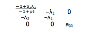
which a33=eT (HessH-λ₁Hessf₁-λ₂Hessf₂-λ₃HessK)e

Because we have S₂=R₂=0, the vectors e₁=(0, 1, 0, 0, 0, 0), e₂=(0, 0, 0, 0, 1, 0) always lie in TQ³. It remains to find an additional vector in TQ³ orthogonal to e₁, e₂ and gradients H, f₂ that we called it e.

G has one zero eigenvalue corresponds to the fact that the Hessian of H is degenerate along the direction tangent to the critical circle. Two other eigenvalues have the similar sign depends on different values of the parameter β and the variables S_i, R_i. This verification checked for a lot of values of β, S_i, R_i. On the basis of this experimental statement we carry out the result.

Theorem 8: In the system, for α =0, the molecule W has the form

A-A for any connected component of Q³. This components can be of the type S_³, RP³. The marked molecule has the following form:

A-A with r=0 for S³,

A-A with r=1/2 RP³.

The mark ϵ depends on the choice of orientation on Q³.

According to proposition there are no saddle critical circles,the molecule W has the form A-A for each connected component of the iso-energy-manifold. The mark r is calculated by using proposition 4.3 of which proves generally the same statement.

References

1. Akbarzadeh, Rasoul, and Ghorbanali Haghighatdoost. "The Topology of Liouville Foliation for the Borisov-Mamaev-Sokolov integrable Case on the Lie Algebra so (4)." Regular Chaotic Dynamics 3 (2015): 317-344.

   [Crossref] [Googlescholar] [Indexed]

2. Bolsinov, Alekseĭ Viktorovich, and Anatolij Timofeevič Fomenko. Integrable Hamiltonian Systems: Geometry, Topology, Classification. CRC Press 2004.

   [Crossref] [Googlescholar]

3. Bolsinov, Aleksei Viktorovich, Sergei Vladimirovich Matveev, and Anatoly Timofeevich Fomenko. "Topological Classification of Integrable Hamiltonian Systems with Two Degrees of Freedom. List of Systems of Small Complexity." Uspekhi Matematicheskikh Nauk 45 (1990): 49-77.

   [Crossref] [Googlescholar] [Indexed]

4. Dullin, Holger, and Vladimir S Matveev. "A New Integrable System on the Sphere." Math Res Lett 11, (2004): 715-722.

   [Crossref] [Googlescholar]

5. Haghighatdoost, Gorbanali, and Andrey A Oshemkov. "The Topology of Liouville Foliation for the Sokolov Integrable Case on the Lie Algebra so (4)." Sbornik: Math 200 (2009): 899-921.

   [Crossref] [Googlescholar] [Indexed]

6. Moskvin, Yu. "Topology of the Liouville Foliation on a 2-Sphere in the Dullin-Matveev Integrable Case." Sbornik: Math 199 (2008): 411-448.

   [Crossref] [Googlescholar] [Indexed]

7. Selivanova, Elena. "New Examples of Integrable Conservative Systems on S2 and the Case of Goryachev-Chaplygin." Commun Math Phys 207 (1999): 641-663.

   [Crossref] [Googlescholar] 

8. Valent, Galliano. "On a Class of Integrable Systems with a Cubic First Integral." Commun Math Phys 3 (2010): 631-649.

   [Crossref] [Googlescholar] [Indexed]