Method - (2022) Volume 11, Issue 8
Received: 04-Aug-2022, Manuscript No. JACM-22-74877;
Editor assigned: 06-Aug-2022, Pre QC No. P-74877;
Reviewed: 12-Aug-2022, QC No. Q-74877;
Revised: 18-Aug-2022, Manuscript No. R-74877;
Published:
24-Aug-2022
, DOI: 10.37421/2168-9679.2022.11.488
Citation: Shaikh, Saad F. “Recurrence Relation When Solving 2nd Order Homogeneous Linear ODEs by Frobenius Method.” J Appl Computat
Math 11 (2022): 488.
Copyright: © 2022 Shaikh SF. This is an open-access article distributed under the terms of the Creative Commons Attribution License, which permits unrestricted use, distribution, and reproduction in any medium, provided the original author and source are credited.
The Frobenius method, also known as the Extended Power Series method comes into play when solving second-order homogeneous linear ODEs having variable coefficients, about a singular point. The solution is expressed in terms of infinite power series. This straightforward article is merely aimed to lucidly arrive at the recurrence relation/formula by taking proper heed of summation limits and simply manipulating them, which is probably absent in almost all research articles and books. The methodology discussed is followed by a few conspicuous and relevant observations.
ODE • Recurrence relation • Singular point • Power series • Homogeneous • Frobenius method
The 2nd order homogeneous linear Ordinary Differential Equations (ODEs) find their applications in several fields of discipline, such as thermodynamics, theory of vibrations, electrical engineering, medicine, etc. [1]. The Frobenius method becomes handy when the ODE is quite complex and consists of variable coefficients. Second-order linear ODEs such as Legendre’s differential equation and Bessel’s differential equation are solved using the Frobenius method, wherein a formal power series solution is obtained.
The Frobenius method is a generalization of the usual power series method. The power series method is applicable when the functions P (x) and Q (x) in the equivalent normalized ODE are analytic x. Therefore, singularity ceases and x0 becomes the ordinary point of the ODE. If one wants to seek an infinite power series solution about point x0 valid in some deleted interval 0 < |x – x0| < R, R being the radius of convergence (R > 0), and x0 as the regular singular point, then the solution y (x), according to stated theorem [2], takes the form,
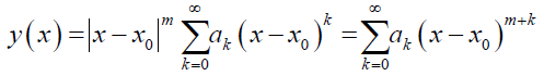
where, ak ≠ 0, m = real or complex definite constant, which can be determined from the indicial equation obtained by equating the lowest power of x in the substituted equation to 0.
This short article is centered around how the lower summation limit and exponent of x alter when the assumed solution, y(x) taken about any regular singular point, x0 is subjected to mathematical operations such as differentiation, multiplication, etc., and how the recurrence relation is obtained by straightforward manipulation of those limits. This is ignored in, principally textbooks [2-12] and open works of literature [13-24]. The recurrence formula, thus obtained is employed to figure out the coefficients (ak) of the powers of x in the final series solution. The methodology is discussed in the subsequent section, followed by useful observations. Few examples have been taken from renowned books for illustration purposes. It is worthwhile to note that not the complete solution is presented, rather important steps up to the recurrence relation are jotted down.
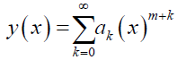
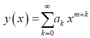
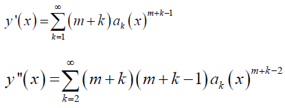
Let the solution y (x) about x0 = 0 be
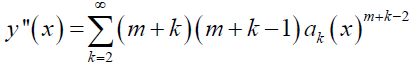
Now, if y (x) is differentiated w.r.t. x, the lower limit of summation will increase by the number of times y (x) is differentiated. Also, the power of x will reduce by the number of times y (x) is differentiated. If y (x) differentiated twice, then
When y (x) is multiplied by xn, where n ϵ N, the lower limit of summation will decrease by the amount n, and the power of x will increase by n. Suppose y (x) is multiplied with x2, then
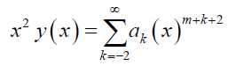
The lower limit of summation reached a value less than 0 i.e., k < 0. In fact, it's not a matter of concern, this is done just to arrive at the recurrence relation, which will be apparent in the forthcoming examples. The following Table 1 summarizes the same. The ODEs normally involve differentiation and multiplication, thus, integration and division can be neglected. Some examples to illustrate the process follows. The solution, y (x) is assumed about x0 = 0 which will be the regular singular point in these examples.
Problem #1 – 3 x y’’ + 2 y’ + y = 0 (1)
Solution. Let
Here, P (x) and Q (x) are not analytic at x = 0; but x P (x) and x2 Q (x) are analytic. Thus, x0 = 0 is the regular singular point, and there exist two nontrivial linearly independent solutions of the given ODE. Depending upon the nature of the roots (m1 and m2) of the indicial equation associated with x0, and the difference between the two roots (m1 – m2), the two linearly independent solutions can be found.
Now,
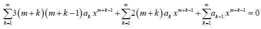
Plugging y, y’, and y’’ into (1), we obtain
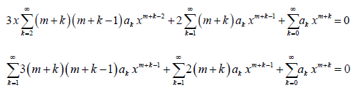
The lower limit of summation and the power of x in the 1st summation above is changed as per Table 1. Upon combining the coefficients of xm + k– 1 (lowest power) in the above equation and setting k = 0, one can obtain the indicial equation, which can be solved for roots, m1, and m2. In the 3rd summation, we set k = k – 1; in order to make the exponent of x the same in all the terms.
Now, all the terms in the above equation have the same summation limits and exponent of x. Thus, we can rewrite it as
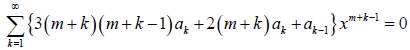
The equation above is much simplified and we can obtain the recurrence formula by equating the coefficient of xm + k – 1 to 0. Therefore,
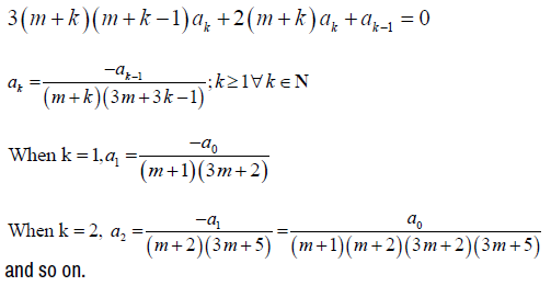
One can proceed by substituting the m values so found, and obtaining the final solution, y (x) in terms of two linearly independent solutions, y1 (x) and y2 (x), based upon the roots of the indicial equation.
| Parameters | Differentiation | Multiplication | Integration | Division |
|---|---|---|---|---|
| Lower limit of summation | Increase | Decrease | Decrease | Increase |
| Power of x | Decrease | Increase | Increase | Decrease |
Problem #2 – 2 x2 y’’ + x y’ + (x2 – 3) y = 0 (2)
Solution. Here, P (x) and Q (x) are not analytic at x = 0; but x P (x) and x2 Q (x) are analytic. Thus, x0 = 0 is the regular singular point, and there exist two nontrivial linearly independent solutions of the given ODE.
Replacing y, y’, and y’’ found in the previous problem into (2), we obtain
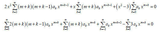
The lower limits of summations and the powers of x in all the summations above are changed as per Table 1. Upon combining the coefficients of xm+ k (lowest power) in the above equation and setting k = 0, one can obtain the indicial equation, which can be solved for roots, m1, and m2. In the 3rd summation, we set k = k – 2; in order to make the exponent of x the same in all the terms.

Now, all the terms in the above equation have the same summation limits and exponent of x. Thus, we can rewrite it as
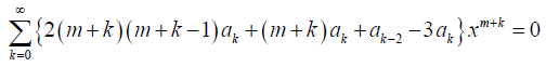
We can obtain the recurrence formula by equating the coefficient of xm + k to 0. Therefore,
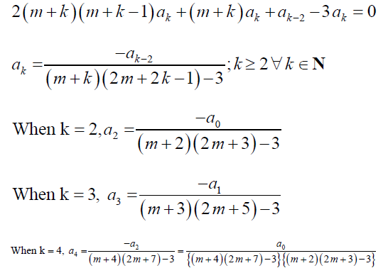
and so on. One can proceed by substituting the m values so found, and obtaining the final solution, y (x) in terms of two linearly independent solutions, y1 (x) and y2 (x), based upon the roots of the indicial equation. Now, the following problem, in fact, is a special case with m = 0, i.e. no singular point exists, and the problem can be solved by the ordinary power series method. Hence, the Frobenius method generalizes the power series method.
Problem #3 – y’’ + x y’ + (x2 + 2) y = 0 (3)
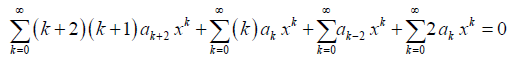
Solution: Here, P (x) and Q (x) are analytic Ɐ x as they are polynomial functions. Thus, x0 = 0 is the ordinary point, and there exist two nontrivial linearly independent power series solutions of the given ODE. These power series converge in some interval |x – x0| < R (R > 0) about x0. Substituting y, y’, and y’’ found in the previous problem into (3), we obtain
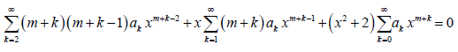
As m = 0, the above equation reduces to
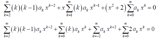
The lower limits of summation and the powers of x are altered in the summations 2nd, 3rd, and 4th above as per Table 1.
In the 1st summation, replace k with (k + 2), and k with (k – 2) in the 3rd summation; in order to make the exponent of x the same in all the terms. This yields
Now, all the terms in the above equation have the same summation limits and exponent of x. Thus, we can rewrite it as
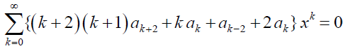
We can obtain the recurrence formula by equating the coefficient of xk to 0. Therefore,
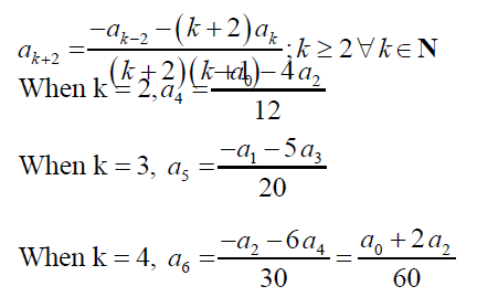
and so on. One can proceed by substituting the coefficients so found, and obtaining the final solution, y (x) in terms of a0, a1, a2, and a3.
Few simple noteworthy observations can be made. Only the exponent of x has to be taken care of before the equating-coefficient step. The summation limits automatically get adjusted by minute alteration, and the summation can be collected as common from all the terms present in the equation. One does not have to expand the series, or through inspection, arrive at the recurrence relation. It can easily be achieved by slight manipulation of the summation limits, for the sole purpose to match the powers of x in the terms, before the equating-coefficient step. The number of coefficients with which the final solution shall be expressed in terms of, can be found out by computing the difference between the smallest and the largest subscripts in the recurrence formula. For instance, in example #3, the number of coefficients which y (x) will be expressed in terms of = |subscript (ak + 2) – subscript (ak – 2) = |k + 2 – k + 2| = 4. However, the more the difference, the more the number of coefficients y (x) will be expressed by, hence, the solution would become quite complicated. Thereby, sometimes expanding the series and later deriving the recurrence formula could assist in developing a link/relation between the coefficients which y (x) is expressed in terms of, resulting in y (x) being expressed in terms of less number of coefficients, hence making the final solution less complex.
It is discernible how smoothly one can arrive at the recurrence relation and compute the required coefficients of x without much painstaking expansion of the summations. However, it is deduced that it could lead to a marginally more intricate solution, since the end result, in certain cases, have to be expressed more in terms of the unknown coefficients.
Funding
The author has no relevant/non-relevant financial interests to disclose.
Conflicts of Interest
The author has no conflicts of interest to declare that are relevant to the content of this article.
Data Availability Statement (DAS)
Data sharing does not apply to this article as no datasets were generated or analyzed during the current study.
Journal of Applied & Computational Mathematics received 1282 citations as per Google Scholar report