Review Article - (2020) Volume 14, Issue 1
Received: 26-Feb-2020
Published:
17-Mar-2020
, DOI: 10.37421/1736-4337.2020.14.297
Citation: Opara, Uchechukwu. “On the Eight Dimensional Point Symmetries of Second Order Linear O.D.E's.†J Generalized Lie Theory Appl 14
(2020): 297. doi: 10.37421/GLTA.2020.14.297
Copyright: © 2020 Opara U. This is an open-access article distributed under the terms of the Creative Commons Attribution License, which permits unrestricted use, distribution, and reproduction in any medium, provided the original author and source are credited.
The purpose of this paper is to review Sophus Lie's methods for differential equations, shedding light on the Lie point symmetries of generic linear second order ordinary
differential equations (O.D.E's). As a matter of necessity in the overall review, there are important contrasts highlighted in derivations of the infinitesimal generators, with and
without the prior application of point transformations.
Lie groups • Lie algebras • Linearizable second order ordinary differential equations • Kummer-liouville point transform • Semi-invariants
The technique of Lie group theory in resolution of differential equations is relatively modern. Sophus Lie, the originator of this technique, developed its foundations very late into the nineteenth century. The theorems discovered by Lie on second order ordinary differential equations are actually classical; with consequences harnessed by Kummer and Liouville [1,2], creating prospective gateways into functional analytic research (consider the necessity to find the kernel of the Kummer-Liouville transform addressed in the relevant section ). As recently as the late twentieth century, there has been a resurgence of attempts to prove a reduction theorem by Lie for linearizable second order O.D.E's (see Results section below for the theorem). Take as an example, the publication by Govinder and Leach [3]. The popular attempts encountered in academic archives fall short of rigorous descriptive detail. This paper offers a well-detailed proof of the above mentioned reduction theorem, with a rare, tactfully systematic and didactic approach.
Given an nth order O.D.E f(x, y, y’(x),…, y(n)(x))=0, there could possibly exist a non-trivial, non-degenerate map on its domain of definition (x, y) ↦ (X, Y) such that we have also f(X, Y, Y’(X),…, Y(n)(X))=0. If there exists a one-parameter family of such maps (Pλ)λ∈R :(x, y) ↦ (X(λ), Y(λ)) such that the following properties hold-
1. Pλ2 ∘ Pλ1=Pλ2 + λ1
2. P0=Identity
3. Pλ is infinitely many times differentiable with respect to x, y and λ,
then we say that the family { Pλ} is a one-parameter symmetry Lie group of transformations that is accommodated by the O.D.E. (X(λ), Y(λ)) is referred to as the global form of the group, and the corresponding infinitesimal form:
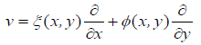
called an infinitesimal generator for the group is obtained by setting
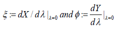
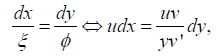
Given the infinitesimal form, we can as well deduce the global form by integrating the autonomous system of differential equations
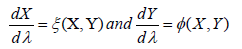
subject to the initial conditions 
Symmetry considerations of differential equations usually simplify these problems, by illuminating their reducibility properties. The method of symmetry groups for differential equations gives rise to certain solutions called group invariant solutions, which may or may not be the entire solution set [4]. The most general technique for discovering Lie symmetries of an equation is by prolonging the infinitesimal vector field action into a jet space. For the case of the O.D.E f(x, y, y(x)’ ,…, y(n)(x))=0,
the jet space will be an open subset of R 2+n, in which we will have the prolonged vector field action
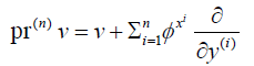
The prolonged vector field action on the jet space gives an induced invariance on that space from the underlying O.D.E. For details on how the algorithm to compute the coefficients φxi is derived, we refer the reader to [5]. Generally, the implementation of this prolongation technique in resolution of O.D.E's involves intuitively equating coefficients of monomials from the process, in line with the theorem given below.
Prolongation theorem Olver [5]
Let f(x, y, y’(x),…, y(n)(x))=0, be an O.D.E that is defined over an open subset M⊆R2. If G is a local group of transformations with infinitesimal generator v acting on M and pr(n)v[ f(x, y, y’(x),…, y(n)(x))]=0 whenever f(x, y, y’(x),…, y(n)(x))=0, then G is a symmetry group of the O.D.E.
It is substitution of the initial variables with the canonical co-ordinates of the accommodated one-parameter symmetries that simplifies a given differential equation. The pair of canonical co-ordinates (μ, ψ) must satisfy μ(X, Y)=μ(x, y) and ψ(X, Y)=ψ(x, y) + λ. The functions μ and ϕ(μ) for any real-valued analytic function ϕ are called invariants of the group.
Much work has been done on symmetry considerations in the specific case of linear second order O.D.E's. For instance, we have explicit derivations of eight independent accommodated infinitesimal symmetries [6]. Detailed account of the crucial Kummer-Liouville transform which pertains to this class of equations [1]. In the ensuing content of this paper, the importance of semi-invariants of the generic equation is frequently brought up. This is an aspect required in obtaining a quality overview of the symmetries, which often tends to be overlooked. Hence, a rare and accurate proof of Sophus Lie's theorem on linear second order O.D.E's is systematically constructed.
The relevance of Lie symmetries in resolution of higher order O.D.E's is then briefly discussed in conclusion.
Point symmetries without point transformations
The equation under examination throughout this section will be the homogenous equation

We need not include the case where a1 and a0 are both constants, which is immediately resolved by means of the characteristic quadratic equation. Although the generic case in non-homogenous, the superposition principle for linear O.D.E's emphasizes the need for solving (1). Solutions to (1) exist locally whenever

for an open, non-empty subinterval (I) of the real number line, so we take this as given a-priori.
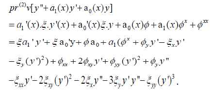
Let ‘v’ be a vector field  defined on some open subset U ⊆ I × R. The second prolongation of ‘v’ is given as
 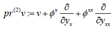 .
.
By the given prolongation theorem, equation (1) accommodates ‘v’ if
 whenever
 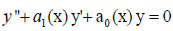 ,
,
in which case ‘v’ is referred to as an infinitesimal Lie symmetry of (1). The collection of all infinitesimal symmetries accommodated by a differential equation forms a linear space referred to as a Lie algebra. Symmetry considerations of (1) arise from the need to simplify or give more elaborate procedures for computing its solutions, and this leads us to implement the prolongation technique for differential equations. To this end, we compute the coefficients φx and φxx respectively to be

The symbol ‘D’ stands for the total derivative, subscripts of ξ and φ symbolize partial derivation, and otherwise, subscripts denote total derivation with respect to the given variables. We will now go into considerable detail on how to compute the infinitesimal symmetries (or generators) of (1) directly. First of all, we determine that
Imposing that (1) accommodates ‘v’, we use the symmetry condition 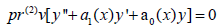 whenever,
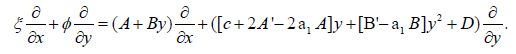
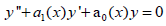 to determine further that
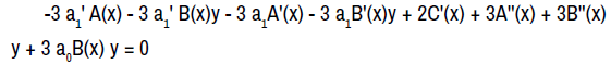
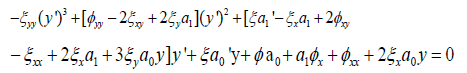
Because the coefficients from the infinitesimal generators do not depend on derivatives of y, we set the coefficients of (y’)3 , (y’)2 and y’ above each equal to zero to realize three equations. A fourth equation also arises by way of the other terms.
From the coefficient of (y’)3, we have 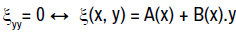 .
.
From the coefficient of (y’)2, we have

From the coefficient of y’,
giving two consequential equations;
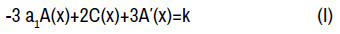

from the free terms and coefficients of y respectively, where k is a constant in (I). Afterwards, the terms from the symmetry condition which are not multiplied by y′ yield three more consequential equations;


Equations (II) and (III) are both derived directly from the adjoint of the original equation (1), that is,

By straightforward computations involving (I), equation (IV) can be reduced to the conditions
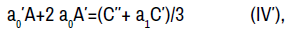

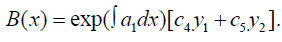
At this juncture, we have obtained sufficient information to tell the most general appearances of the coefficient functions from the infinitesimal symmetries. Let the constant k in (I) be denoted c1. In (V), we determine that D(x)=c2y1+c3y2, where y1 and y2 are specific linearly independent solutions of (1). From (II′), we have
To solve for A(x), it is helpful to examine the normal form of (1), that is,
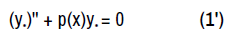
obtained via the point transform

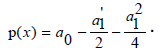
Hence, the coefficient of y* in the normal form, which is identified as the semi-invariant of (1) is given as,
 Therefore, we can rewrite (IV′′) as A''' + 4pA' + 2p'A = 0. It is then easy to check that y*1 . y*2 is a solution to (IV'') where y*1 , y*2 are both solutions to the normal form of (1). Therefore, we determine the most general solution to the third order linear O.D.E (IV'') to be:

This is substituted in (I) to give

Hence, we obtain the most general point symmetry of (1), without any prior point transformation, to be
After substituting the values obtained above, we can separate the most general symmetry by the eight constants {ci}8i=1 as follows:

Suggestive of an eight-parameter symmetry group of (1). The process of computing the symmetries as done above for this case turns up an obvious problem: almost all the single-parameter symmetries depend on having a specific solution y1 or y2 of (1) in hand a-priori. The only single-parameter symmetry which does not depend on any specific solution is  , which corresponds to the so called scaling group. It is accommodated by all linear differential equations. In this study, the scaling group reduces (1) to a Riccati equation of the first order, when applied alone. We observe this development by computing the global form of this one-parameter group to be
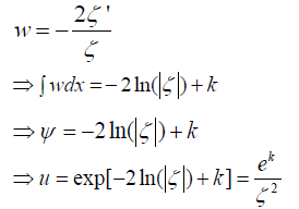
and then a canonical co-ordinate for the group is ψ = ln y because  Substituting the dependent variable in (1) with the canonical co-ordinate, we obtain the first order non-linear Riccati equation
 where w = Ψ ' .
In fact, there is also a reverse correspondence in this regard, being that every Riccati equation can be transformed into a linear O.D.E of the second order.
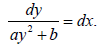
We will hereby make a few further remarks on Riccati equations, as they are relevant to this study. Special Riccati equations have the form
where a, b, α are real constants. When α = 0, the special Riccati equation is integrated by separation of variables:
Another easily solved case is α=-2, in which substitution of the dependent variable z=1/2 maps the above Riccati equation to the form
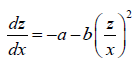
which can then be integrated by quadrature. Riccati and Bernoulli both discovered that the special Riccati equation can be mapped to the form wherein α=0, and can hence be integrated by quadrature in terms of elementary functions, if α takes values in one of the two rational sequences
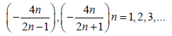
The limit of both of these sequences is -2. Later, Liouville showed that these Riccati equations can be mapped to a form that can be integrated by quadrature in terms of elementary functions only if α takes a value in one of these two rational sequences.
In the case of a general Riccati equation

it is linearizable by a point transformation of the dependent variable y to a linear O.D.E of the first order, if and only if it has a constant solution [7]. More details on the simplification and integration of such O.D.E's can be readily accessed, but we now return our focus to point symmetries of (1).
To modify the result on symmetries of (1) obtained prior to remarks on Riccati equations, there are point transformations which we may implement before employing the prolongation technique. The most general point transformation which preserves the order and linearity of (1) is called the Kummer-Liouville (KL) transformation, and we will unravel more subtle properties of the infinitesimal symmetries by engaging it.
Point symmetries with KL point transforms
The Kummer-Liouville transform is given by

which rearranges (1) to be of the form

Where J is an open, non-empty sub-interval of the real number line.
Theorem (Stackel - Lie) [1]
The Kummer-Liouville transform is the most general point transform which preserves the order and linearity of (1).
For clarity, we will use the prime sign (' ) to denote differentiation with respect to x and an overset dot to denote differentiation with respect to t. Observe that we need the following three to occur in order to obtain (2) from (1) by way of transform (KL).
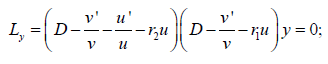
(i) We must have the non-commutative factorization

where r1 (t) and r2 (t)satisfy the Riccati equations:

The reduction of (1) to (2) was posed as Kummer's problem, which was to find the set of all KL transformations that could do this. It is known that Kummer's problem is always solvable. As a combination of the above three requirements for the KL transform, we get that (1) can be reduced to (2) if and only if the following two conditions are satisfied
where
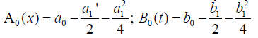
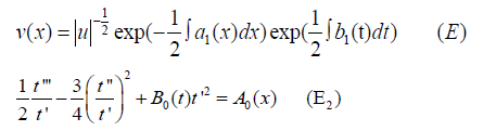
are respectively called the semi-invariants of (1) and (2). We solve (ii) over v in order to get (E) and then we substitute (iii) by (E) using the relation u=t′ to get (E2).
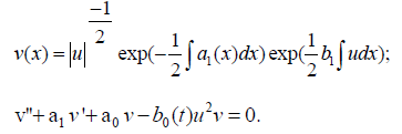
At the crux, we wish to reduce (1) to a linear O.D.E of autonomous form, that is, one with constant coefficients;
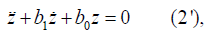
where the coefficient b0 is a real number, while b1 may either be real or purely imaginary.
(2′) can be factorized either through the noncommutative operators of the first order-
or through the commutative operators of the first order-

Where r1, r2 are roots of the characteristic equation; r2+b1r+b0=0.
We remark that (1) can be reduced to (2') by transform KL if and only if the following occur.
(i) (1) admits a certain one-parameter Lie symmetry
(ii) u(x) satisfies 
(iii) 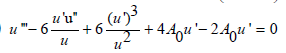
(iv) The multiplier v and the kernel u of the KL transform are related through the formulas
(v) The resolvent of (2') is given by the function

and it satisfies
(vi) 
The one-parameter existence follows from the reducibility of (1) to autonomous form (2'), as will soon be discussed. Condition (iii) can be obtained from (ii) by calculation, and then (vi) can be obtained from (iii) by way of the resolvent function

To be substituted in the resolvent function, we have linearly independent solutions of (1) given by
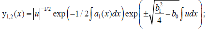
for the case of KL transform to autonomous form (2') .
Focusing now on the general symmetry of (2), we must recall the KL substitutions
y=vz, t=∫udx, so as to observe that
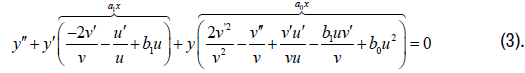
By applying the second prolongation under the condition b0′= b1′=0, we realize that (3) admits the infinitesimal generator
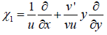
which precisely corresponds to the case of reduction to autonomous form (2'). Thus, the canonical coordinates for χ1 are made of the pair (t, z), where z:=y/v is called an invariant and t=∫ udx. The invariant is obtained by integrating the differentials
Resulting in y/v=constant, which is why y/v is an invariant. The other canonical coordinate is simply
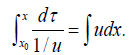
Since the pair of canonical coordinates results in the reduction of (1) to autonomous form, the Lie symmetry χ1 is the requirement addressed in condition (i) above. Involving the autonomous case, equation (3) yet again accommodates an eight-parameter Lie symmetry, and so seven other independent single-parameter symmetries besides χ1 are mentioned as follows:
The linear space spanned by χ1 to χ8 is a Lie algebra that is stable under the Lie bracket structure [.,.] as shown in the table included below Table 1. Instability under the Lie bracket or commutator would have implied the necessity to include more vector fields, other than  , to the infinitesimal generators spanning the Lie algebra accommodated by (3). This is at large, due to the fact that O.D.E's only accommodate finite dimensional Lie algebras. The element in the i'th row and j'th column of the table is the vector field [χi, χj].
| χ1 | χ2 | χ3 | χ4 | χ5 | χ6 | χ7 | χ8 | |
| χ1 | 0 | 0 | χ1 | χ2 | 0 | 0 | 2χ3+χ6 | χ5 |
| χ2 | 0 | 0 | 0 | 0 | χ1 | χ2 | χ4 | χ3+2χ6 |
| χ3 | -χ1 | 0 | 0 | χ2 | -χ5 | 0 | χ7 | 0 |
| χ4 | -χ2 | 0 | -χ2 | 0 | χ3-χ6 | χ4 | 0 | χ7 |
| χ5 | 0 | -χ1 | χ5 | χ6-χ3 | 0 | -χ5 | χ8 | 0 |
| χ6 | 0 | -χ2 | 0 | -χ4 | χ5 | 0 | 0 | χ8 |
| χ7 | -2χ3-χ6 | -χ4 | -χ7 | 0 | -χ8 | 0 | 0 | 0 |
| χ8 | -χ5 | -χ3-2χ6 | 0 | -χ7 | 0 | -χ8 | 0 | 0 |
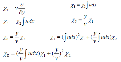
Note that the characterization of Lie brackets [X, Y] f = X(Y(f)) - Y(X(f)) for 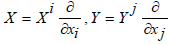 and any C∞ function f gives us the formula:

The Lie brackets of the infinitesimal symmetries in their initial computed forms  are not so readily determined. Nevertheless, the symmetries
 can be obtained as linear combinations of
  from functional specifications for the kernel (u) and multiplier (v) stated above. For instance, we have the chiefly required symmetry for conversion to autonomous form obtained as:
Although the KL transform gives more insight into the symmetry concept being addressed, all the infinitesimal generators except χ6 (which corresponds to the scaling group) depend on the special kernel function u, and this is still indirectly tantamount to solving (1) beforehand. For this reason, construction of algorithms for computing the kernel has a substantial heuristic value in itself.
It is useful to engage a second point transformation to (1) in discussions of its Lie symmetries, which is the reduction to normal form. After the generic KL transform, we reduce (2) into normal form by changing the dependent variable to ͞z where
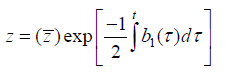
and the result of this transform is
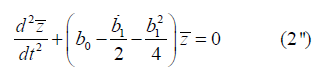
where  has previously been identified as a semiinvariant of (2). Having presented sufficient pertinent information, this particular transform is geared towards validating Sophus Lie's theorem on linear O.D.E's of the second order, as stated below.
Theorem (Lie's theorem on linear second order O.D.E's) [8]
The O.D.E (1) can be mapped via a point transform into the form  , which implies accommodation of the eight-dimensional Lie algebra sl(3,R).
Now, we can map (1) into the above mentioned form from (2'') by finding which value of u solves B0=0. What we obtain concretely is

In (2'') after a double point transformation of (1). The details for justification of this transformation are given below.
By setting the semi-invariant of (2) equal to zero, we get the semiinvariant of (1) to be
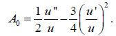
It is clear that the associated homogenous equation A0=0 accommodates the scaling group, of which the global form is Pλ(x,u)=(x,eλu), so we obtain a canonical coordinate for this one-parameter group to beψ = ln (u) .Recall the condition that u ≠ 0 on the interval I of interest. If u is negative then ψ = ln ( u ) ,and this sign change will not tamper significantly with the result of the ensuing computation. Consider the first case,

and we have the following simplification for the semi-invariant of (1);

where  . The equation given just above is a Riccati equation, so we hereby employ the correspondence between Riccati equations and second order linear O.D.E's. By substituting w with
  , the Riccati equation becomes
 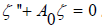 .
.
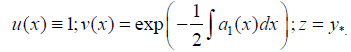
This linear equation is always solvable for  in C2(I), from which we recover u by reversing the prior substitutions as shown below.
where k is a constant of integration and ζ is a non-trivial solution to (1'). This given value of u solves B0=0.
We should remark that the transform from (1) into its own normal form (1') is only a particular case of the (KL) transform with the functions
Therefore, the kernel u of transform KL enables us to restructure the Lie symmetries of (1), so as to reduce this O.D.E into various simpler forms. We can take u as the auxiliary variable to examine the two most important cases; namely b0′= b1′= 0 for reducibility of (1) to autonomous form, and B0=0 for reducibility of (1) to the form  , which corroborates Sophus Lie's theorem.
As a further remark, it is noteworthy that an arbitrary O.D.E of the second order is linearizable if and only if it accommodates an 8-parameter symmetry group, which is the symmetry group of maximal dimension for this class of equations. If it does accommodate such a group, then it can be mapped by point transformation(s) to the equation . If it does not accommodate a symmetry group of dimension 8, then it accommodates a 0-, 1-, 2-, or 3-parameter symmetry group. This is another aspect of Sophus Lie's categorization of second order ordinary differential equations. For example, as we have seen above, the non-linear differential equation involved in the semi-invariant of (1), which is given as 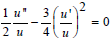 , is linearizable. The Lie algebra of infinitesimal symmetries accommodated by this equation is spanned by the eight vector fields listed as follows.

It is befitting to pass a few further comments on point symmetries of O.D.E's of order three and higher, following the details elucidated on those of the second order. For each given order, there is a maximal dimension for admissible symmetry groups [9], such as is eight for equations of the second order. Whenever an O.D.E admits a Lie group of one-parameter symmetries of the maximal dimension, then it is linearizable by a point transformation. Moreover, whenever the canonical coordinates from an accommodated one-parameter symmetry are employed by change of variable(s), the original O.D.E is transformed into another form with order one less. For instance, we have already seen as an explicit application of the scaling group in transforming the second order equation (1) into a firstorder Riccati equation.
The main challenge that lingers in the midst of an abundance of oneparameter symmetries is that, whenever a given equation is reduced to another form by any one of them, the resulting form usually fails to inherit any of the symmetries which were present at first [10]. To simplify further using the Lie symmetry technique, one would then have to perform the infinitesimal symmetry prolongations again, which may or may not yield any vector fields. Not every differential equation admits a Lie symmetry to begin with, and computer algebra is encouraged for equations with order three or higher due to the rapid growth of the number of computations involved with each increment in order (and degree) of the differential equations. These signal a number of pronounced limitations involved with the approach of Lie groups. Nevertheless, whenever present, the wieldiness of Lie symmetries provides several opportunities for greater in-depth study of differential equations at large, as exemplified above.