Research - (2022) Volume 16, Issue 9
Received: 09-Sep-2022, Manuscript No. GLTA-22-74228;
Editor assigned: 13-Sep-2022, Pre QC No. P-74228;
Reviewed: 02-Nov-2022, QC No. Q-74228;
Revised: 04-Nov-2022, Manuscript No. R-74228;
Published:
11-Nov-2022
, DOI: 10.37421/1736-4337.2022.16.347
Citation: Almutiben, Nouf, Edward L. Boone, Ryad Ghanam and G. Thompson. “Lie Symmetries of the Canonical Connection: Codimension Two Abelian Nilradical.” J Generalized Lie Theory App 16 (2022): 347.
Copyright: © 2022 Almutiben N, et al. This is an open-access article distributed under the terms of the Creative Commons Attribution License, which permits unrestricted use, distribution, and reproduction in any medium, provided the original author and source are credited.
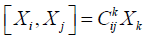
In this paper we study the Lie symmetries of the canonical connection on Lie groups for the special case when the Lie algebra has a codimension
two abelian nilradical. In this particular case, we have only one algebra in dimension four, namely A4,12 and three algebras in dimension five; namely  . For each of these algebras we investigate and classify the symmetry algebra associated with its geodesic equations.
Lie group • Canonical connection • Geodesic system • Lie symmetry
This article is concerned with the canonical symmetric connection ∇ associated to any Lie group G. It was introduced originally in 1926 as the “zero”-connection; see [1]. Some properties of ∇ are considered in Helgason S [2]. More recently ∇ and its geodesic system have been investigated within the context of the inverse problem of Lagrangian dynamics; see [3-7]. There has also been a lot of work related to the symmetry analysis of the geodesic equations in lower dimensions [8-11].
In this paper we focus our study on the symmetry analysis of
the geodesic equations of the canonical connection for the special
case when the niradical of the Lie algebra is two-dimensional ableian
algebra. In dimension four there is only one Lie algebra of this type;
namely A4,12 and in dimension five there are three families of Lie
algebras Lie algebras with parameters- with this property; namely; . In Section 2, we define and prove all the
geometric properties of the canonical connection on Lie groups [12].
In Section 3, we consider the algebra A4,12 we derive the geodesic
equations from a basis of right-invariant vector fields representation
of the Lie algebra. We also compute a basis of the symmetry Lie
algebra and analyze its Lie algebra.
Similarly, in Section four we consider the three five-dimensional
Lie algebras .
Finally, regarding our notation, we will use (x, y, x, w, p, q) are our
coordinates. We will denote 
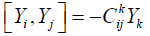
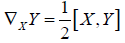
On left invariant vector fields X and Y the canonical symmetric connection ∇ on a Lie group G is defined by
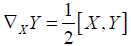 (2.1)
(2.1)
and then extended to arbitrary vector fields using linearity and the Leibnitz rule. Clearly ∇ is left-invariant. One could just as well use right-invariant vector fields to define ∇, but one must check that ∇ is well defined, a fact that we will prove next.
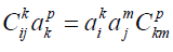
Proposition 2.1
In the definition of ∇ we can equally assume that X and Y are right-invariant vector fields and hence ∇ is also left-invariant and hence bi-invariant. Moreover ∇ is symmetric, that is, its torsion is zero.
Proof
The fact that ∇ is symmetric is obvious from eq. (2.1). Now we
choose a fixed basis in the tangent space at the identity TIG. We shall
denote its left and right invariant extensions by {X1, X2,..., Xn} and {Y1,
Y2,..., Yn}, respectively. Then there must exist a non-singular matrix A
of functions on G such that  We shall suppose that
 (2.2)
(2.2)
Changing from the left-invariant basis to the right gives
 (2.3)
(2.3)
Next, we use the fact that left and right vector fields commute to deduce that
 (2.4)
(2.4)
where the second term in 2.4 denotes directional derivative. We note that necessarily
 (2.5)
(2.5)
Now we compute
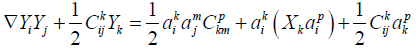 (2.6)
(2.6)
Next we use 2.4 to replace the second term on the right hand side of 2.6 so as to obtain
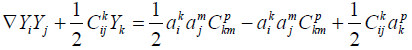 (2.7)
(2.7)
However, the right hand side of 2.7 is seen to be zero by virtue of 2.3. Thus
 (2.8)
(2.8)
whenever X and Y are right invariant vector fields.
An alternative proof of Proposition (2.1) uses the inversion map ψ defined by, for S ∈ G
ψ (S ) = S−1 (2.9)
As such, one checks that ψ∗I maps a left-invariant vector field evaluated at I to minus its right-invariant counterpart evaluated at I. Then ψ∗I is an isomorphism and there is no change of sign in the structure constants, as compared with eq. (2.5). Since there are two minus signs in eq. (2.1) the same condition eq. (2.1) applies also to right-invariant vector fields.
Proposition 2.2
i. An element in the center of g engenders a bi-invariant vector field.
ii. A vector field in the center of g is parallel.
iii. A bi-invariant differential k-form θ is closed and so defines an element of the cohomology group Hk (M,ℝ).
Proof
i. Suppose that Z ∈ TIG is in the center of g and let exp(tZ) be the associated one-parameter subgroup of G so that Z corresponds to the equivalence class of curves [exp(tZ)] based at I. Let S ∈ G; then LS∗Z corresponds to the equivalence class of curves [S exp(tZ)] based at S. Since Z is in the center of g then exp(tZ) will be in the center of G and hence [S exp(tZ)]=[exp(tZ)S]. It follows that any element in the center of g engenders a bi-invariant vector field.
ii. Obvious from eq (2.1).
iii. A proof can be found in [13]. Spivak shows that ψ∗ (θ)=(−1) kθ, whereas dθ, which is also bi-invariant, changes by ψ∗(dθ)=(−1)k+1dθ. It follows that dθ=0.
Proposition 2.3
i. The curvature tensor, which is also bi-invariant, on vector fields X, Y, Z is given by
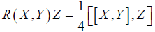 (2.10)
ii. The connection ∇ is flat if and only if the Lie algebra g of G is two-step nilpotent.
iii. The tensor R is parallel in the sense that ∇W R(X, Y)Z=0, where W is a fourth right invariant vector field, so that G is in a sense a symmetric space.
iv. The Ricci tensor Rij of ∇ is given by
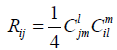 (2.11)
and is symmetric and bi-invariant and is obtained by translating to the left or right one quarter of the Killing form. It engenders a bi-invariant pseudo-Riemannian metric if and only if the Lie algebra g is semisimple.
Proof
i. Is obvious and applies to arbitrary vector fields since it is a tensorial object.
ii. Is obvious.
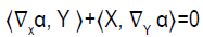
iii. This fact follows from a series of implications:
4∇W R(X, Y)Z+4R(∇W X, Y)Z+4R(X, ∇W Y)Z+4R(X, Y)∇W Z=∇W [[X, Y ], Z] (2.12)
⇒ 4∇W R(X, Y)Z+2R([W, X], Y)Z+2R(X, [W, Y ])Z+2R(X, Y)[W, Z] −1/2[W, [[X, Y ], Z]=0 (2.13)
⇒ 4∇W R(X, Y)Z+1/2[[W, X],Y],Z]+1/2 [X, [W, Y ]], Z]+1/2 [[X, Y ], [W, Z]]−1/2 [W, [[X, Y ], Z]=0 (2.14)
⇒ 4∇W R(X, Y)Z+1/2 [[W, X], Y ], Z]+1/2 [X, [W, Y ]], Z] – 1/2 [Z, [[X, Y ], W]=0 (2.15)
⇒ ∇W R(X, Y)Z=0 (2.16)
iv The formula eq (2.11) is obvious from eqs. (2.1) and (2.10). The last remark follows from Cartan’s criterion.
Proposition 2.4
i. Any left or right-invariant vector field is geodesic.
ii. Any geodesic curve emanating from the identity is a oneparameter subgroup.
iii. An arbitrary geodesic curve is a translation, to the left or right, of a one-parameter subgroup.
Proof
i. Is obvious because of the skew-symmetry in eq (2.1).
ii. By definition the curve t → [S exp(tX)] integrates a geodesic field X.
iii. If the geodesic curve at t=0 starts at S, translate the curve to I by multiplying on the left or right by S-1 and apply (ii).
Proposition 2.5
i. A left or right-invariant vector field is symmetry, a.k.a. affine collineation, of ∇.
ii. Any left or right-invariant one-form engenders a first integral of the geodesic system of ∇.
Proof
i. The following condition for vector fields X and Y says that vector field W is a symmetry or, affine collineation, of a symmetric linear connection:
∇x∇YW−∇xYW−R(W, X)Y=0 (2.17)
In the case at hand of the canonical connection, this condition just reduces to the Jacobi identity when W, X and Y are all left or right-invariant.
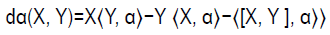
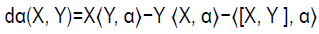
ii. A one-form α is a Killing one-form, if the following condition holds:
 (2.18)
In the case of the canonical connection, if X and Y are rightinvariant and α is right-invariant then eq (2.1) gives
 (2.19)
Clearly, (2.19) implies (2.18) so that every left or right-invariant one-form engenders a first integral of the geodesics: if the one-form is given in a coordinate system as αidxi on G, the first integral is αiui viewed as a function on the tangent bundle T G that is linear in the fibers.
Proposition 2.6
Any left or right-invariant one-form α is closed if and only if ⟨[g, g], α⟩=0, that is, α annihilates the derived algebra of g.
Proof
Consider the identity
 (2.20)
If α is left-invariant and we take X and Y left-invariant, then the first and second terms in eq (2.20) are zero. Now the conclusion of the Proposition is obvious. The proof for right-invariant one-forms is similar.
Proposition 2.7
Consider the following conditions for a one-form α on G:
i. α is bi-invariant.
ii. α is right-invariant and closed.
iii. α is left-invariant and closed.
iv. α is parallel.
Then we have the following implications: (i), (ii) and (iii) are equivalent and any one of them implies (iv).
Proof
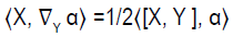
The fact that (i) implies (ii) and (iii) follows from Proposition (2.2) part (iii). Now suppose that (iii) holds and let X and Y be right and leftinvariant vector fields, respectively. Then consider again the identity
 (2.21)
Assuming that α is closed, then either because [X, Y]=0 or by using Proposition 2.6, we find that eq. (2.21) reduces to
X⟨Y, α⟩=Y ⟨X, α⟩ (2.22)
Now the left hand side of eq.(2.22) is zero, since Y and α are left-invariant. Hence ⟨X, α⟩ is constant, which implies that α is rightinvariant and hence bi-invariant. Thus (iii) implies (i). The proof that (ii) implies (i) is similar.
Finally, supposing that (ii) or (iii) holds we show that (iv) holds. Then as with any symmetric connection, the closure condition may be written, for arbitrary vector fields X and Y, as
⟨∇Xα, Y ⟩−⟨X, ∇Y α⟩=0 (2 .23)
Clearly eq (2.18) and eq (2.23) imply that α is parallel. So a closed, invariant one-form is parallel.
Of course, it may well be the case that there are no bi-invariant one-forms on G, for example if G is semi-simple so that [g, g]=g. However, there must be at least one such one-form if G is solvable and at least two if G is nilpotent. If we choose a basis of dimension dim g-dim [g, g] for the bi-invariant one-forms on G, it may be used to obtain a partial coordinate system on G, since each such form is closed. Such a partial coordinate system is significant in terms of the geodesic system, in that it gives rise to second order differential equations that resemble the system in Euclidean space.
Proposition 2.8
Each of the bi-invariant one-forms on G projects to a one-form on the quotient space G/[G, G], assuming that the commutator subgroup [G, G] is closed topologically in G. Furthermore the canonical connection ∇ on G projects to a flat connection on G/[G, G] and the induced system of one-forms on G/[G, G] comprises a “flat” coordinate system.
Proof
The fact that a bi-invariant one-form on G projects to a one-form on G/[G, G] follows because each such form annihilates the vertical distribution of the principal right [G, G]-bundle G → G/[G, G] and furthermore the equivariance, or Lie-derivative condition along the fibers, is trivially satisfied since the one-form is closed. The fact that ∇ projects to G/[G, G] follows because [G, G] ◁ G, as was noted in Šnob L and Winternitz P [14].
The Four-Dimensional Lie Algebra A4,12
In this section we consider the only four-dimensional Lie algebra with co-dimension two nilradical. This Algebra is denoted by A4,12 and the non-zero brackets are given by
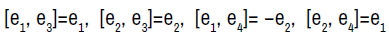 (3.1)
(3.1)
A vector field representation of the above algebra is given in terms of right-invariant vector fields as follows [3]
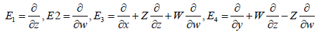 (3.2)
(3.2)
It is easy to verify that the commutators of the above vector fields give the same relations as equation 3.1
Geodesic equations
In this section we consider the system of geodesic equations of the canonical connection on Lie groups. Given an n-dimensional Lie algebra g, the system of geodesic equations is given by
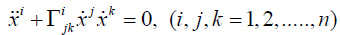 (3.3)
(3.3)
Now, we compute the geodesic equations for the Lie algebra
A4,12. In order to calculate the connection components  , we need
to calculate the covariant derivatives of the vector fields given by
eqn. (3.2). We will also use the definition of the canonical connection
given by eqn. (2.1). This will result in a system of equations with to be the unknowns. To illustrate this, we will show how to obtain one
equation in the system. For example:
, we need
to calculate the covariant derivatives of the vector fields given by
eqn. (3.2). We will also use the definition of the canonical connection
given by eqn. (2.1). This will result in a system of equations with to be the unknowns. To illustrate this, we will show how to obtain one
equation in the system. For example:
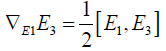 (3.4)
(3.4)
The left hand side of eqn. (3.4) gives the following
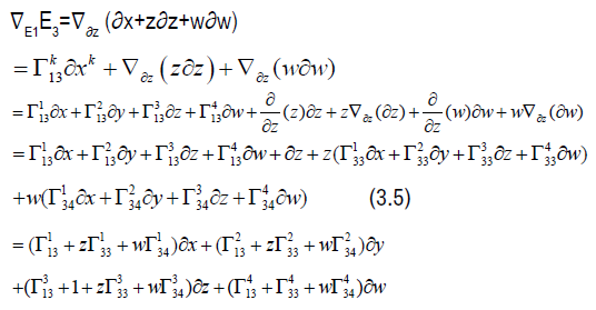
The right hand side of eqn. (3.4) gives
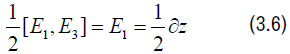
and so equating the sides give the following equation:
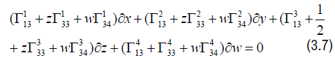
and so we obtain the following system of equations:
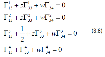
After we apply all covariant derivatives and use the definition of the canonical connection we obtain the following components of the connection given by:
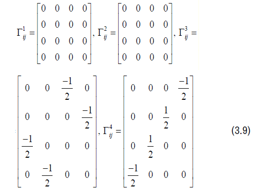
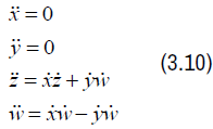
Therefore we obtain the following system of geodesic equations:
The lie symmetry algebras
The symmetry Lie algebra for the geodesic equations is given by:
The non-zero Lie brackets of the symmetry algebra is given by:
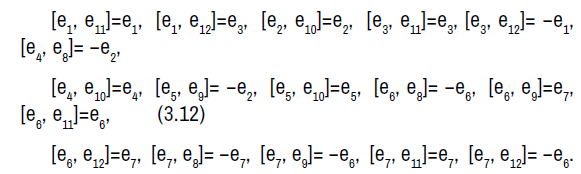
The symmetry algebra is a solvable Lie algebra with sevendimensional abelian nilradical spanned by e1, e2, e3, e4, e5, e6, e7 and a five-dimensional abelian complement spanned by e8, e9, e10, e11, e12.
In this section we consider the five dimensional Lie algebras with co-dimension two abelian nilradical. There are only three algebras;
 .
.
Algebra 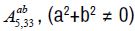 . The non-zero brackets for the algebra
  are given by
 (4.1)
(4.1)
The geodesic equations are given by
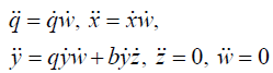 (4.2)
(4.2)
We now consider the following subcases depending on the values of a and b:
The non-zero brackets of the symmetry algebra is given by:
The non-zero brackets of the symmetry algebra is given by:
The non-zero brackets of the symmetry algebra is given by:
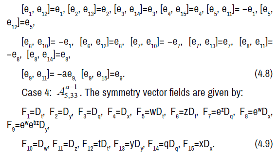
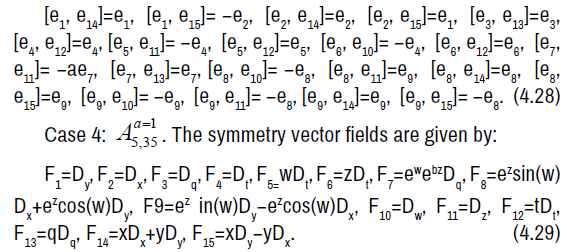
The non-zero brackets of the symmetry algebra is given by:
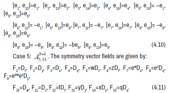
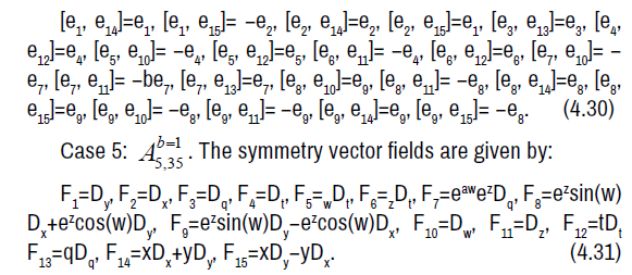
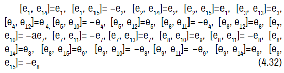
The non-zero brackets of the symmetry algebra is given by:
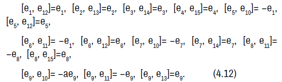
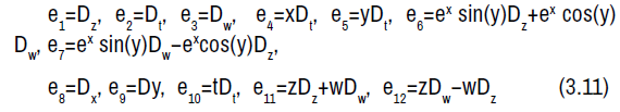
The symmetry Lie algebra is a fifteen-dimensional solvable Lie algebra with nine-dimensional nilradical spanned by e1, e2, e3, e4, e5, e6, e7, e8, e9 and an abelian six-dimensional complement spanned by e10, e11, e12, e13, e14, e15.
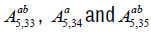
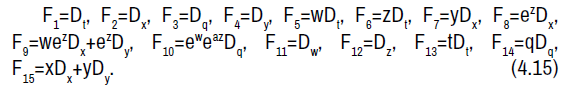
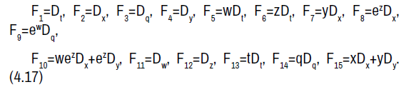
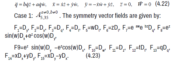
Algebra  . The non-zero brackets for the algebra Aa5,34 are
given by:
. The non-zero brackets for the algebra Aa5,34 are
given by:

The geodesics equations are given by:
 (4.14)
We now consider the following subcases:
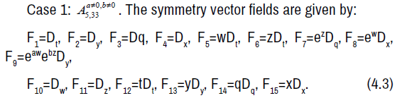
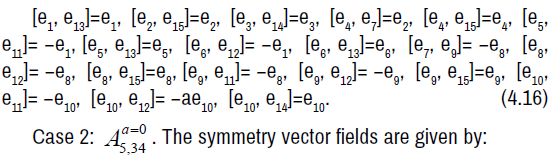
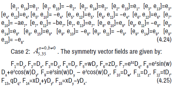
Case 1:  . The symmetry vector fields are given by:
The non-zero brackets of the symmetry algebra is given by:
The non-zero brackets of the symmetry algebra is given by:
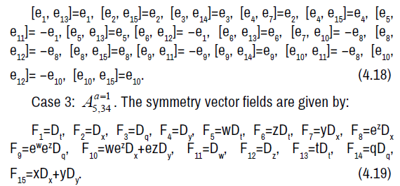
The non-zero brackets of the symmetry algebra is given by:
The symmetry Lie algebra is a fifteen-dimensional solvable Lie algebra with a ten-dimensional nilradical spanned by e1, e2, e3, e4, e5, e6, e7, e8, e9, e10 and an abelian five-dimensional complement spanned by e11, e12, e13, e14, e15.
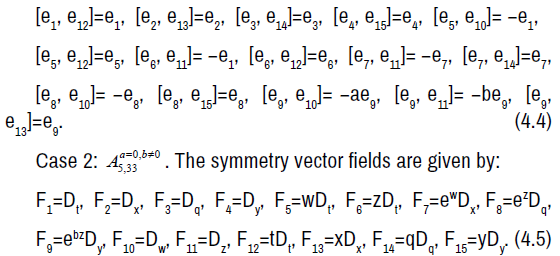
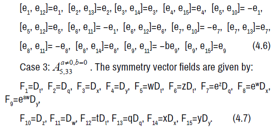
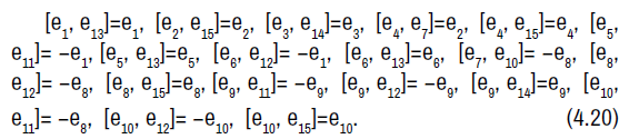
Algebra  . The non-zero brackets for the algebra (a2+b2≠0) are given by:

The geodesics are given by:
The non-zero brackets of the symmetry algebra is given by:
The non-zero brackets of the symmetry algebra is given by:
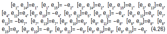
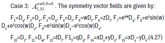
The non-zero brackets of the symmetry algebra is given by:
The non-zero brackets of the symmetry algebra is given by:
The non-zero brackets of the symmetry algebra is given by:
The symmetry Lie algebra is a fifteen-dimensional solvable Lie algebra with a nine-dimensional nilradical spanned by e1, e2, e3, e4, e5, e6, e7, e8, e9 and an abelian six-dimensional complement spanned by e10, e11, e12, e13, e14, e15.
Nouf Almutiben would like to thank Jouf University and Virginia Commonwealth University for their support. Ryad Ghanam would like to thank Qatar Foundation and Virginia Commonwealth University in Qatar for their Support.
No conflict of interest.
Google Scholar, Crossref, Indexed at
Google Scholar, Crossref, Indexed at
Google Scholar, Crossref, Indexed at
Google Scholar, Crossref, Indexed at
Google Scholar, Crossref, Indexed at
Google Scholar, Crossref, Indexed at
Google Scholar, Crossref, Indexed at
Google Scholar, Crossref, Indexed at
Google Scholar, Crossref, Indexed at
Google Scholar, Crossref, Indexed at