Individual Preferences and the Growth Dynamics of Two Political Parties: Insights through a Simple Mathematical Model

Joseph Frank Gordon^1* and Farai Nyabadza^2
*Correspondence: Joseph Frank Gordon, Department of Mathematical Sciences, African Institute for Mathematical Sciences, Biriwa, Ghana, Email:

Keywords

Mathematical model • Equilibria • Stability • Political parties • Epidemic approach

Introduction

A political party is an organisation of people which seeks to achieve common goals to its members through the acquisition and exercise of political power. A main feature of political parties is that they are composed of factions; groups of politicians or party members who differ in their ideological views. Many of these political parties have an ideological core, but some do not, and many represent very different ideologies than they did when first founded [1]. Political parties are the hallmark of democracies. In every democratic regime, groups establish these institutions. In democracies, political parties are elected to run a government through competitive elections. An election is a decision-making process by which a population chooses an individual to hold formal office [2]. The constitution of Ghana provides a single citizenship for the whole nation and provides every citizen of Ghana of 18 years of age or above and of sound mind, the right to vote and is entitled to be registered as a voter for the purpose of public elections. Ghana’s public elections are usually based on the single vote method where every registered voter votes for one presidential candidate who wins upon receiving the highest number of votes in a given election. In most democratic countries like Jamaica, Malta, Ghana and the United States, there exist only two party systems where two political parties dominate to such an extent that electoral success under the banner of any other party is almost impossible. In a situation where smaller parties exist, such parties can join any of the dominant parties based on their ideological core [1]. In every democratic country, members of political parties contact registered voters from other political parties and individuals from the voters class with the hope of convincing them to join their party [3]. Individual preferences for a particular political party over other political parties usually depends on the type of interactions the person has with individuals in another party and the person’s background. According to Carol et al. (2007) [4], one major contributing factor in an individual’s decision to change his or her voting class is one’s personal influence. This includes the person’s religious values, their socio-economic status, their family upbringing and their cultural values. As said by Tom W. Rice (1985) [5], personal influence also includes the incumbency factor since whether a candidate has already been a president affects how a person views that candidate. Personal obligations also affect the level of individual preferences for a particular party. For instance, individuals who are very busy at work or home may choose to become less active (weak preference) in politics or to the extent of not voting on the election day since they are too busy to meet personal obligations. In the same vein, since the movement of people from their political party to another party has become very common these days, people leave their party and join another party due to the fact that some people may not be comfortable with the changes occurring in their party and as a result may prefer the next dominant party to the previous party. Again, individuals may also change their preference over a particular party based on the fact that he or she has realized that other members in the other party receive proper weight or position in their party better than what they get in their own party. It has been these attributes about political parties that have driven many political scientists to study the components that lead to individual preferences and the growth dynamics of political parties due to the movement of people among such parties. With this in mind, mathematical models have been constructed or created to study such social phenomena using the tools used to model epidemic models. Khan (2000) [6], modeled a multiparty political system with time delay in switching. In this model a political system with three political parties and a group of non-affiliated voters were considered. In his model, he considered four coupled non-linear ordinary differential equations in which members of the third party change allegiance and after a time delay become an active member of one of the other parties. Equilibrium and stability analysis were also carried out. It was showed that Hopf bifurcation can occur where all political parties will survive undergoing regular fluctuations as a result of taking time delay as a bifurcation parameter. Findings in this paper showed that, the group of parties having majority will rule the country and next will sit in opposition. The rest of the political parties and independent elected members come under the third party. This implies that members of the third party defect towards the ruling party due to self interest and after a lapse of some time, became active members of that party. Huckfeldt and Kohfeld (1992) [7], examined the electoral stability and dynamic consequences of the decline in class based democratic politics by considering two political parties. In their paper, two different mathematical models were constructed: a system of a linear differential equations assuming behavioural independence within the electorate and a system of non-linear differential equations assuming behavioural interdependence. In both models, the movement from one political party to the other party were also taken into account. In the above models, the epidemic approach were not used in the modelling process, howewer, Calderon et al. (2005) [8], studied non-linear mathematical model for the spread of third parties ideologies in a voting population where they assumed that party members are more influential in recruiting new third party voters than non-member third party voters. The use of epidemic approach in modeling process of political parties was applied in their model since political party members make door-to-door campaigning with the hope of convincing people to vote for their party. In their model, the role of two other major parties in the political system were not considered as they really focused on the expansion of the third party. In their simplified model, they considered three classes namely people who vote but not to third parties, those who vote for third party and party officials and donors were also taken into consideration. In their general model, they divided the susceptible class and voters class into two parts on the basis of low and high affinity to the third party’s ideology. Belenky and King (2007) [9], in their model considered the US federal election in which candidates from two major political parties compete for votes of undecided voters in a state who usually do not vote in US elections. They also considered in their model, the margin of votes to be received from such voters by either candidate as a result of the election campaign of all the competing candidates. Kaare Strom (19901) [10], studied the behavioral theory of competitive political parties by considering three models of competitive political party behavior namely the vote-seeking party, the office-seeking party and the policy-seeking party. However, his model suffer from various theoretical and empirical limitations and the conditions under which each model applies were not also well specified. Further studies can be done to cater for these limitations and to some extent well defined conditions for the three models. Gilat Levy (2004) [11], in his paper studied the model of political parties. In his paper, he assumed that the role of parties is to increase commitment ability of politicians through the voters. Whereas a politician running alone can only offer his ideal policy, the set of policies that a party can commit to is the support of its members. Findings showed that the commitment mechanisms provided by the institution of parties has no effect when the policy space is uni-dimensional; the policies parties can induce in equilibrium arise also when politicians are running independently. However, when the policy space is multidimensional, politicians use the vehicle of parties to offer equilibrium parties that they cannot offer in their absence. Michael Laver (2007) [12], in his paper studied an agent based model on the choice of citizens of parties so support in elections. He also studied the choice of party leaders of policy ”packages” offered to citizens in order to attract this support. The agent based model was then extended to deal with the birth and death of political parties treating the number and identity of political parties as an output of, rather input to, the process of party competition. The party birth was modeled as an endogenous change of agent type from citizen to party leader, which described the citizen dissatisfaction with the history of the system. Aggregate outputs were also measured in terms of the mean and standard deviation of citizens’ distances from their closest party. The key parameter in their model was the survival threshold meaning that citizens left on average less dissatisfied with lower threshold and vice versa. In this paper, we consider a non-linear mathematical model for the spread of two political parties, the ruling party and the opposition. We use the principles borrowed from infectious diseases modeling to track the changes of the membership of each political party taking into consideration the individual preferences. The inclusion of individual preferences in our model is very important as members in each class make choices depending on their preferences for the political parties. In this project, we assume that registered voters preferences for a political party can take one of these three stances: that is, in a situation where preferences for political parties are weak, where preferences are strong and lastly, where no preferences have been made by individuals. In a situation where preferences are weak, individuals do not actively promote the growth of their political parties. Thus, individuals plan to vote for the political party only on the election day. Such people do not campaign, advertise, put up posters neither will they initiate any political discussion about the presidential election with other individuals in any way. Preferences of individuals for a political party are deemed as strong when individuals plan to vote for the party and actively support it. Such individuals try to convince other people to vote for their party through rallies, advertisement and other means to get people vote for their party. Individuals with no preferences are those that remain undecided as to which political party to vote for. In the present paper, we assume that individuals of voters class are susceptible to both political parties, like in epidemics, where two infective class and one susceptible class have been considered, see [13]. Recruitment of new voters and the movement of voters between political parties remain a common phenomena in modern democracies. In this paper, we are motivated by the work presented in [3] to consider recruitment of new members to political parties while considering their preferences. Our work follows the work in [3] but is motivated in adding choices made by individuals, which is an integral part in decision making when joining a political party [14]. As a result, the specific aims include:

1. Reformulating the model in [3] to include individual preferences.

2. Carrying out the stability analysis of the steady states.

3. Carrying out the numerical simulations.

This paper is motivated by the work in [3]. We now give the model formulation where we will then include our modifications.

Model Formulation

Let N be the total population considered in the system, which is assumed to be constant and homogeneously mixed. The total population is divided into three classes namely (i) the voter’s class V (ii) Political party B, and (iii) Political party C. We assume that the per capita exit rate is the same as the per capita recruitment rate. Our population is thus considered to be constant. Let μ be the rate at which individuals enter or leave the voting system. Then we define μN as the rate at which individuals enter the voters class. Due to in-activeness and death, individuals leave the political system at a rate μ for each class. In the modeling process, individuals in the voter’s class can join either political party B or C depending on their choice. It is also important to consider the possible interactions that can occur among individuals, the rate at which these interactions occur as well as the effect that the interaction has on the individuals involved. So we have that the members of both political parties contact individuals of V and convince them to join their party. Based on the interactions that occur among individuals, individuals in the V class may decide to join party B at a rate of β₁V (B/N), where β₁ is the per capita recruitment rate in party B. The parameter β₁ is the effective contact rate. That is, the contacts that result in an individual joining a political party. It is often a product of the probability that a contact will result in recruitment and the number of contacts made. Similarly, individuals in V may also decide to join party C at the rate of β₂V (C/N), where β₂ is the per capita recruitment rate in party C. The parameter β₂ is the effective contact rate. That is, the contacts that result in an individual joining a political party. It is often a product of the probability that a contact will result in recruitment and the number of contacts made. We assume that individuals leave their political party to join the other political party when influenced by members of either party. So we let θ₁ and θ₂ be the per capita recruitment rate from B to C and from C to B respectively. Thus, members in party B may join party C at the rate of θ₁B(C/N) and similarly, members in party C may also join party B at the rate of θ₂C(B/N).

The flow diagram of the model is shown in Figure 1 below.

Using this idea to build expressions relating to the transition between classes, we construct a mathematical model governed by the following differential equations as follows:

(1)

subject to the initial conditions V (0)>0,B(0) ≥ 0 and C(0) ≥ 0. The above system is presented and analysed in [3].

We seek to modify the contact functions and in this work. Summing the above equations in (1) gives

which shows that our population is constant over time and V+B+C=N. Thus, we can choose to ignore one of the variables. It is often convenient to consider fractions of a population rather than the whole population numbers. We achieve this mathematically by normalizing our equations in (1) and renaming variables to represent fractions of the overall population. We define the quantity v=V/N where v represents the proportion of the total population that belongs in the voters class. Similarly, we can define b=B/N to be the proportion of the population in political party B and c=C/N denoting the proportion of the total population that belongs in political party C. Substituting these normalized variables into our system reduces (1) to the following form:

(2)

In (2), β₁b and β₂c are replaced by following preference functions

(3)

(4)

A plot of the function in (3) for different parameter values of α1 is shown below

Similary, a plot of the function in (4) for different parameter values of α2 is also shown below

Here α_1,2, denotes the preference for political party B and C respectively. So our model reduces to the one in [3] if α_1,2=1. If α_1,2=0, then no preferences are made by individuals and as a result, no transfers occur from the voters class, V. From the above plots, if α_1,2 ∈ (0,1), then we have reduced the recruitment into B and C and this is referred to as weak preferences by individuals. Again, if α_1,2 ∈ (1,∞), then this model increased preferences. This is called strong preferences by individuals. Now using this modification, (2) can be written as

(5)

Now the above system (5) contains three equations and since our total population is constant over time and V+B+C=N, this gives v+b+c=1 which implies we can reduce our system to two dimensions using the substitution v=1−b−c into equation (5). Now considering the per capita recruitment rate from political party B to C, θ₁ and per capita recruitment rate from political party C to B, θ₂, we consider the net shifting of members from party B to C or vice versa. So we let θ=θ₁−θ₂ where without loss of generality we assume that θ>0 as in [3]. This assumption means that the net shifting of party members is from political party B to political party C. Using these facts, the reduced model system (5) will be given by the following two differential equations:

(6)

The study of (6) is equivalent to the study of the model system (5). Keeping this in view, we study the model system (6). The governing equations in the model system (6) are also consistent with the ones in ecological models. We now analyze the above system (6) using tools used for ecological models and interpret the result in terms of the political dynamics.

Equilibrium Analysis

To capture the long term dynamics of political parties B and C, we carry out the stability analysis of the steady states. Now to solve for the equilibrium points, we solve these two equations

(7)

(8)

Our model admits four equilibrium points discussed below.

E₁:Party Free Equilibrium (PFE)

The party-free equilibrium (PFE) for our reduced system occurs at (0,0), the steady state achieved when the entire population resides in the voters class and where there are no individual preferences for political parties since no political parties exist. The PFE is essentially analogous to the disease-free equilibrium in epidemic models and always exists as a possible outcome for the voting class. This is sometimes called the nonpartisan system where no official political parties exist, sometimes reflecting legal restrictions on political parties. In nonpartisan elections, each candidate is eligible for office on his or her own merits [1]. So E₁=(0,0).

E₂:Single Party B Equilibrium (SPE)

Now to obtain the single-party equilibrium for our reduced system, we solve the following equations. From (7) and (8), we have

Now with c=0, the above equation reduces to

Now in solving for b in the above equation, we obtain the equilibrium point

with Now for this equilibrium point to make political sense, then it existence is subject to the condition R₁>1. This condition ensures the survival and existence of political party B where the members of political party C are zero. It also shows the preferences individuals have for such party when party C does not exist.

Theorem 3.1. The equilibrium point E₂ exists only if R₁>1.

E₃: Single Party C Equilibrium (SPE)

Similarly, from (7) and (8), we obtain the other single-party equilibrium points by solving the following equations:

Now with b=0, the above equation reduces to

Now in solving for c, we get the equilibrium point

(9)

with Now for this equilibrium point to be politically relevant, then its existence is subject to the condition R₂>1. This condition ensures the survival and existence of political party C where the members of political party B are zero. It also shows the preferences individuals have for such party when party B does not exist.

Theorem 3.2. The equilibrium point E₃ exists only if R₂>1.

The equilibrium E₂ and E₃ are referred to as single-party equilibrium. In single-party systems, one political party is legally allowed to hold effective power. Although minor parties may sometimes be allowed, they are legally required to accept the leadership of the dominant party. The single-party system is sometimes equated with dictatorship and tyranny. North Korea and China are examples of such system [1].

E₄: Interior Equilibrium

The interior equilibrium is synonymous to the endemic equilibrium in disease epidemics. Now to obtain the interior equilibrium point, we solve these two equations

(9)

(10)

Now expanding (9) and (10), we obtain the following set of equations:

(11)

(12)

where

But we have that and hence (11) and (12) now becomes

(13)

(14)

Now solving for b in (13), we obtain

(15)

Now we substitute (15) into (14) to get the equation

m₂c²+m₁c+m₀=0,

whose solution is given by

where

Thus c=c± where

Hence we have the interior/endemic equilibrium as

The above equilibrium suggest the co-existence of the two parties. These equilibrium basically explain individual preferences for either political party and their existence. In such situation we have that the two political parties dominate the whole population of the country with individual members supporting either party strongly. We can comprehensively investigate the interior equilibrium through numerical simulation due to the mathematical complexity of the interior equilibrium Figures 2 and 3.

Stability Analysis of Steady States

In order to analyze stability, we linearise the system and compute partial first derivatives with respect to each of the variables b and c. Jacobian for the reduced system: Now considering the differential equations below

We let:

and

Then, the general Jacobian matrix J of the above set of differential equations is given by

where

Now we investigate the stability analysis of the various equilibrium by finding values of the above Jacobian matrix evaluated at the each of the equilibrium points.

Party-Free Equilibrium (E₁)

Applying the above reduced Jacobian matrix to our PFE, (0,0) where we only consider b and c terms, we determine PFE stability as follows:

It is clearly seen that the eigenvalues of the above Jacobian matrix are λ₁=βˆ ₁α₁-μ which implies μ(R₁−1) and λ₂=βˆ ₂α₂−μ which also implies μ(R₂−1). If R₁<1 and R₂<1, then the given values λ₁ and λ₂ are both negative and positive otherwise. We can summarize these findings in the following theorem.

Theorem 4.1. The equilibrium point E₁ is locally asymptotically stable if R1<1 and R2<1 and unstable otherwise.

Single-party Equilibrium (E₂) The Jacobian matrix for the single party equilibrium is given by

It is clearly seen that the eigenvalues of the above Jacobian matrix are

and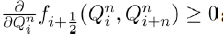

The eigenvalue λ₁ is always negative and the eigenvalue λ₂ is negative only if R₂<1 and θ<μ and positive otherwise.

Theorem 4.2. The single party equilibrium E₂ is locally asymptotically stable if R₂<1 and θ<μ. It is unstable otherwise.

Single-party Equilibrium (E₃) Now considering the single party equilibrium 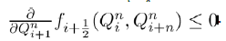then the Jacobian matrix is given by

It is clearly seen that the eigenvalues of the above Jacobian matrix are

and

The eigenvalue λ₁ is always negative and the eigenvalue λ₂ is negative if R₁<1. So we summarize these findings in the following theorem.

Theorem 4.3. The single party equilibrium E₃ is locally asymptotically stable if R₁<1 and unstable otherwise.

As suggested earlier, we would carry out numerical simulation to show the co-existence and the stability nature of our interior equilibrium in the next section.

Numerical Simulations

In every epidemiological model, numerical simulations are carried out in order to explain and confirm the analytical results. So to check the feasibility of our analytical results regarding the existence conditions and stability of our steady states, we carried out some numerical simulations by intuitively using hypothetical values for our parameters in (6) since realistic data are not available. Now due to the size of the mathematical expressions of our interior equilibrium, we have carried out numerical analysis to show its existence and its stability. Figure 4, shows the variations of political party B and C with respect to time. This basically explains the co-existence of the two political parties. From the above figure, it is easy to note that both political parties started with the same number of members but for some time political party B leads over political party C in terms of number of members indicating high recruitment rate and high preferences of individuals for party B. But after some time, political party C leads over party B in the long-run. The system settles to a steady state in which political party C dominates. We now present the result depicted by Figure 4 as a phase portrait. We thus use the same parameter values in the caption of Figure 4 to obtain the following diagram. Figure 5 shows the phase diagram for b and c. The diagram shows the existence of a stable steady state E₄ with the rest of the steady states being unstable. The stability of E₃ is numerically represented by Figure 6. We thus give both the time series plot and the phase diagram Figure 7. From Figure 6, It is easy to note that, both political parties have started with the same number of members but for some time, both political party B and C decreases and in the long-run only political party C remains stable whiles party B dies out. The system settles to a steady state in which political party C dominates. From Figure 7, it may be noted that all the trajectories are approaching to political party C showing that political party C remains stable in the long-run as already shown in Figure 6. The stability of E₂ is numerically represented by Figure 8. We thus give both the time series plot and the phase diagram Figure 9. From Figure 8, It is easy to note that both political parties, B and C started with the same members, but for some period of time, party B decreases and eventually increases in the long-run. Party C on the other hand decreases and eventually dies out in the long-run as party B becomes stable in the long-run. From Figure 9, it is clearly shown that all the trajectories are approaching party B explaining it stability in the long-run whiles party C dies out. The stability of the nonexistence of both parties E₁ is numerically represented by Figure 10. We thus give both the time series plot and the phase diagram 11. From Figure 10, it is easy to see that both political parties decreases with respect to time and dies out in the long-run. Irrespective of the preferences individuals have for either party, both parties die out in the long-run. As clearly seen from Figure 11, the trajectories approach zero showing the non-existence of both parties in the long-run as depicted in 10. In model system (6), we have made the graphs of variation of political party B with respect to time for different values of α1. From Figures 12 and 13, It is clear that as the value of α1 increases irrespective of the interval it lies, the members of political party B increases showing that as the preferences of individual increases, members of political party B increases and vice versa. Similarly, the same result holds in the case of political party C taking into consideration different values for α₂.

Conclusion

In this paper, we proposed and analysed a model, which is a modification of an epidemiological type non-linear mathematical model for the spread of two political parties presented in [3]. The modification was done by incorporating individual preferences in individuals as they make choices between the two political parties. We have analyzed the steady state of political importance namely (i) party-free equilibrium, (ii) single-party equilibrium and (iii) numerically the co-existence of the two parties. From the local stability analysis of the steady states, two threshold parameters R₁ and R₂ were obtained. Analysis of the model shows that political party B will die out if R₁<1. Given that implies that . This means that recruitment into political party B is less than the loss of individuals in the same political party. On the other hand, political party C dies out if

Since we assume that θ=θ₁−θ₂ >0, it implies that individuals move from party B to C. So party C only dies out if the recruitment in party C (β₂α₂) is less than the exit into the party but in addition less people must move from party B. The analytic conditions for the co-existence equilibrium could not be determined analytically. We thus resorted to numerical simulations. Various time series plots and phase portraits were plotted to confirm the analytic results. This model may be generalized by considering a multi-party system which may affect the dynamics of the political scenario of any country. People also delay in their preferences for a political party and this model may also be generalized by considering the effect of this time delay involved in preferring one political party to the other. The policy of why people prefer political party B to party C and vice versa was not captured in this model and as a result, future work could be carried out to include such policy.

References

1. Political party. Wikipedia, the Free Encyclopedia. (2015).
2. Democracy. Wikipedia, the Free Encyclopedia. (2015).
3. Misra AK. A simple mathematical model for the spread of two political parties. Nonlinear Analysis: Modelling and Control. 17(2012):343-354.
4. Ambrose C, Jones J, Larson K, Orozco D et al. A mathematical model of political affiliation (2007).
5. Rice TW. Predicting presidential elections: A review essay, (1985).
6. Khan QJA. Hopf bifurcation in multiparty political systems with time delay in switching. Applied Mathematics Letters. 13(2000):43-52.
7. Huckfeldt R and Kohfeld CW. Electoral stability and the decline of class in democratic politics. Mathematical and Computer Modelling. 16(1992):223-239.
8. Calderon K, Orbe C, Panjwani A, Romero DM, et al. An epidemiological approach to the spread of political third parties (2005).
9. Belenky AS and King DC. A mathematical model for estimating the potential margin of state undecided voters for a candidate in a us federal election. Mathematical and computer modelling. 45(2007):585-593.
10. Strom K. A behavioral theory of competitive political parties. American journal of political science, (1990):565-598.
11. Levy G. A model of political parties. Journal of Economic Theory, 115(2004):250-277.
12. 12.Laver M and Schilperoord M. Spatial models of political competition with endogenous political parties. Philosophical Transactions of the Royal Society B: Biological Sciences. 362(2007):1711-1721.
13. Naresh R and Tripathi A. Modelling and analysis of hiv-tb co-infection in a variable size population. Mathematical Modelling and Analysis. 10(2005):275-286.
14. Plumper T and Martin CW. Multi-party competition: A computational model with abstention and memory. Electoral Studies. 27(2008):424-441.