Research Article - (2025) Volume 14, Issue 2
Received: 16-May-2024, Manuscript No. IJEMS-24-135787;
Editor assigned: 21-May-2024, Pre QC No. IJEMS-24-135787 (PQ);
Reviewed: 04-Jun-2024, QC No. IJEMS-24-135787;
Revised: 11-Mar-2025, Manuscript No. IJEMS-24-135787 (R);
Published:
18-Mar-2025
, DOI: 10.37421/2162-6359.2025.14.771
Copyright: © 2025 Bwambok K, et al.. This is an open-access article distributed under the terms of the creative commons attribution license which permits unrestricted use, distribution and reproduction in any medium, provided the original author and source are credited.
The aim of this study was to establish the interlink between inflation rates, interest rates, gross domestic product and oil price movement on the stock market returns. The study aimed to ascertain the reaction of the stock market to a movement in each of the macroeconomic variables. The effect of the movement of oil prices on the stock market returns was also measured. Published time series data from 1990 to 2022 was sourced from the NSE, Kenya National Bureau of Statistics and the Central Bank of Kenya. Empirical results from the regression model concluded that oil price movement displayed a major relationship with stock market volatility. A percentage point movement in the price of oil, the model forecasted stock market return drop of 0.4%. Inflation rates, Interest rates and gross domestic product returned immaterial relationships. The impact of a standard deviation shock on each of the macroeconomic variables on stock market returns concluded that shock in oil prices was both negative and positive confirming their asymmetric relationship.
Oil prices • Macroeconomic variables • Stock market returns
Background of the study
That fluctuating oil costs have an impact on national economies and by extension, stock market returns, is supported by theory. Financial and social stability are very precarious in the face of unpredictable swings in crude oil costs. When the cost of a barrel of oil climbs rapidly and abruptly, it is called an oil price shock. The sudden appearance of a promising new business opportunity may be seen by some as a shock to the price of crude oil.
The study on asymmetric volatility transmission implies that oil price shocks may have a bigger influence on stock market volatility in developing nations than in industrialized ones. This is because emerging countries' economies are less diversified and more dependent on oil imports. Therefore, the economy of developing nations may be hit more by a spike in oil costs. Stock market returns are also not uniformly affected by oil price shocks, with developing countries being more likely to have negative returns than developed nations.
Furthermore, through asymmetric volatility transmission, the volatility of one financial market or asset can affect the volatility of another market or asset in a non-symmetric way. This means that when the volatility of one market or asset increases, the effect on the volatility of another market or asset may be different than when the volatility of the first market or asset decreases. This is predicated on the theory that markets and assets are interrelated and that volatility in one market may bleed over into other markets and impact their respective levels of volatility. This has the potential to trigger the contagion effect, which refers to the propagation of an economic crisis from one market or area to another and may take place on either the national or worldwide level. Global financial markets are interconnected as shown in Figure 1.

Figure 1. Stock market returns in different markets.
Despite trends that show almost near volatilities, underlying factors such as macro-economic policies adopted by the individual economies within which these stock markets are found play a significant role. China as shown, has clear outlier policies or market approaches that resulted in peaks in 2007 and 2015.
Crude oil price shocks
According to the market experiences a shock whenever the price of crude oil rises. Such a rise is often known as "oil price crisis." In the 1970 s, the world was hit by a series of oil price shocks that were generally acknowledged as devastating to economic activity, especially in the developed countries. Most of these jolts may be traced back to swings in oil prices.
"Oil price shocks," as sudden increases or decreases in oil costs are commonly called, have the ability to significantly impact many different businesses (Figure 2).

Figure 2. The trends in oil price shocks from 1970 to 2022.
Oil price shocks, as seen by the graph, have been very unpredictable and fluctuated widely over the last several years. Cost of oil more than quadrupled in response to the 1973 Yom Kippur War, when the OPEC cut off oil shipments to countries that supported Israel. After this, in 1979, there was an oil crisis as a direct consequence of the Iranian Revolution and the start of the Iran-Iraq War, both of which caused costs to quadruple. This was followed by the Gulf War. During the Gulf War that took place between 1990 and 1991, prices increased once again as Iraq invaded Kuwait and threatened to interrupt oil production in the Persian Gulf.
Cost of oil climbed from roughly $30 per barrel in 2003 to over $140 per barrel in 2008 owing to a mix of causes, including rising demand from China and other developing countries, geopolitical tensions and speculation in financial markets. This caused prices to spike from around $30 per barrel in 2003 to over $140 per barrel in 2008. The global oil glut that was created by the US shale oil boom, slowing demand from China and OPEC's decision not to decrease output led to the cost of oil collapse that occurred from 2014 to 2016. During this time, oil cost reduced from $100 per barrel to approximately $30 per barrel. Price fall of oil in 2020 was caused in part by OPEC and Russia's disagreement over whether or not to reduce output in response to the unanticipated drop in demand caused by the COVID-19 outbreak.
Historically, the oil price shocks are confirmed by economic theory where the demand supply elasticity gets exaggerated and distorted after some cyclical shocks like recessions, embargoes, wars, monetary crises and extreme climatic changes.
Oil price shocks and Kenya’s stock market
Kenya's stock market has been facing a challenging environment in recent years, with several factors affecting its performance. The market has been experiencing volatility, with fluctuations in prices and volumes traded. This has led to a lack of investor confidence and reduced trading activity.
When the cost of oil fluctuates, the Kenyan stock market reacts quickly and violently. As a country that must constantly replenish its supply of oil from outside, Kenya's economy is very vulnerable to fluctuations in the global oil market. The higher the cost of oil is, the higher the expenses of manufacturing and transportation are going to be, which may have a detrimental impact on companies and sectors that are dependent on these inputs.
In addition, the instability of oil cost causes uncertainty in the market, which makes it difficult for investors to make choices that are guided by relevant information. This has led to a decrease in investor confidence and reduced trading activity, which has affected the liquidity of the market. Another problem facing Kenya's stock market is the impact of political instability and corruption. These issues have contributed to a lack of investor confidence, with many investors hesitant to invest in a market that is perceived to be unstable.
Overall, the combination of oil price shocks, political instability and corruption has created a challenging environment for Kenya's stock market. Addressing these issues will be crucial to restoring investor confidence and improving stock out-turn.
Stock market volatility is a real possibility because of how sensitive the global economy responds to oil cost movement. This is of utmost importance in nations like Kenya who are very reliant on foreign oil supplies. The Nairobi Securities market, sometimes known simply as the NSE, is the primary securities market in Kenya and is regarded as a vital indication of the fiscal success of the nation.
Statement of the problem
As Herrera and Pesavento point out, the interconnectedness of oil prices, financial markets and the economy has become more important. The influence of oil cost movements on economic activity and the development of macroeconomic policy is generally acknowledged. The 1973 oil crisis prompted academics to study the consequences of unexpected increases in oil prices on the economy. Studies conducted in the past have shown a clear relationship between this phenomenon and a number of important macroeconomic indicators, including inflation, gross domestic product and unemployment. On the other hand, there was some suspicion that these shocks in oil prices also had an effect on other areas, such as the financial markets.
Anand, Sunil and Ramachandran found that fluctuations in the oil market had significant effects on the economy and the stock market both immediately and later on as a result of their impact on other macroeconomic variables. This is due to oil prices' dramatic effect on the economy. However, there hasn't been much research done on how oil price shocks affect the NSE.
To address this information gap, the current study looks at how oil price shocks affect the volatility Kenya's NSE stock market. This research attempts to determine how changes in oil prices affect the volatility of NSE stock returns. The results of this study will provide Kenyan stock market investors, policymakers and others a better understanding of how to protect themselves from the effects of oil price shocks. These findings will be provided as a result of the research that was conducted.
Research questions
Objectives of the study
The overarching purpose of the research is to investigate the effects of fluctuations in the price of oil on the volatility of the stock market traded on the Nairobi Securities Exchange (NSE) in Kenya. The specific objectives are as follows:
Significance of the study
The findings of this study will benefit policymakers, entrepreneurs and anyone with a stake in the Kenyan economy in mitigating the market's negative reaction to oil price shocks. An executive summary will be provided detailing these results.
Scope and organization of the study
This research used quarterly secondary time series data spanning the period from 1990 to 2022 in Kenya. There are three parts to the overall strategy. The first chapter is an introduction that includes a summary of the subject, a statement of the study's purpose, a list of research questions and an explanation of the importance of the study. The second chapter is a literature review, which covers issues including a theoretical overview, empirical studies and a conclusion. In chapter 3, the research methodology is laid out. The research consists of the following sections: Introduction, study design, conceptual framework, model definition, variable measurement, target population, sampling methodology and processes, data kinds, sources and collection methods, study equipment, pilot study and data analysis [1-5].
The present chapter encompasses a comprehensive exposition of the study's design, theoretical framework, empirical models to be estimated, data kind and source, as well as the chosen estimation technique.
Research design
This study will make use of a design that is not experimental since it is the method that is most suited for the variables that are being investigated, which the researcher will not be able to modify or control. The independent variables are not changed in a nonexperimental design; instead, the emphasis is placed on analyzing the way in which the variables naturally interact with one another. This helps to limit the possibility of error and improves the validity of the findings.
Theoretical framework
The rational expectations theory is going to be used as a framework for this research in order to explain the link between oil price shocks and volatility on stock markets, as well as the influence these shocks have on Kenya's inflation rate, interest rates and Gross Domestic Product (GDP).
EGARCH models will be used to assess market and oil price volatility and SEM will be used to investigate the presence of potential causal links between the variables.
Model specification
Examining how changes in oil prices have affected NSE stock volatility is the main objective. The EGARCH model found in equation that has been changed as a result of Molepo in order to reflect returns and volatility in NSE and oil prices. In the same way as VOLNSE represents stock market volatility, VOLOIL represents oil price volatility.
Equation (1) will be used in order to do the estimate of the stock market's volatility.
The oil price shocks will be calculated using equation (2)
Both found that the standard deviations of stock and oil returns fluctuate over time and exhibit heteroscedasticity. This indicates that any conclusion concerning the effect on volatility may be inaccurate if the time dependent feature of volatility is ignored. This is because market volatility increases over time. Volatility variables may respond asymmetrically to shock orientations inside the EGARCH model [5-8].
The conditional variance of returns obtained from the maximum likelihood estimate of an EGARCH (0,1) model is used to mimic the volatility of shocks in the NSE and 0il prices.
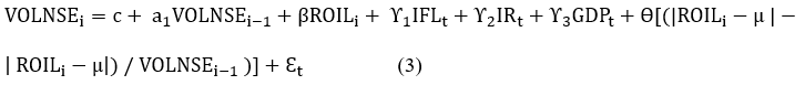
Where, C represents the intercept term, capturing the baseline or constant level of stock market volatility that is not accounted for by the other variables in the equation. VOLNSEi represents the logarithmic form of the stock market volatility at time i. VOLNSEi-1 represents the lagged stock market volatility at time i-1. ROILi represents the logarithmic form of oil price shocks at time i. ROILi-1 represents the lagged oil price shocks at time i-1. IFLi represents the inflation rate at time i. IRi represents the interest rate at time i. GDPi represents the GDP growth rate at time i. α1 is the coefficient of the lagged stock market volatility, representing the persistence or autocorrelation of volatility over time. β1 is the coefficient of the lagged oil price shocks, capturing the impact of past oil price shocks on stock market volatility. γ1, γ2, and γ3 are the coefficients associated with each control variable (inflation rate, interest rate, and GDP growth rate), representing their respective impacts on stock market volatility. θ represents the coefficient associated with the leverage effect term, which captures the asymmetric response of volatility to oil price shocks. [(|ROILi-μ|-|ROILi-μ|)/VOLNSEi-1] denotes the leverage effect term, where |ROILi-μ| derives the absolute difference between the oil price shock at time i and its mean (μ) and | ROILi-μ| subtracts the absolute difference from itself, displaying the asymmetry. This term is scaled by VOLNSEi-1 to include the effect of past volatility on the current leverage effect and εi denotes the error term, displaying the unexplained variation in the stock market volatility equation at time I [6,7].
Definition and measurement of variables
The description and measurement of variables is explained in Table 1 as shown.
| Type | Variable | Definition of variable | Measurement of variable |
| Dependent variables | VOLNSE |  |
Changes in the FTSE-NSE 25 index |
| ROIL | 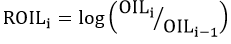 |
London's commodities exchange crude oil price index is used to generate oil price returns | |
| Independent variables | INFL | Persistent increase in general prices of goods and services | ΔLn CPIt=LnCPIt-LnCPIt-1 |
| IR | Interest rate | LnIRt percentage | |
| GDP | Total market value of final output produced within a country | LnGDPt |
Table 1. Definition and measurement of variables.
Data type and source
The research will use time series data acquired from many sources including the NSE, OPEC, Brent, Platts Crude pricing, and EPRA [8-11].
Data analysis
Before the model was estimated and in order to guarantee that no erroneous diagnoses are made, diagnostic tests were performed. The tests include; stationarity test, co-integration test, diagnostic test, normality test and correlation test. Phillips-Perron test and Augmented Dickey-Fuller test was carried out to ensure that both the mean and variance of the time series data are constant to minimize chances of obtaining spurious results.
Johansen and Phillips-Ouliaris (PO) was used to test the long-haul variable connectivity in non-stationarity data set. Breusch-Pagan test for heteroscedasticity and Goldfeld-Quandt was used to test for homoscedasticity to ensure that the estimated equation gives consistent results over time and Pearson's correlation coefficient (r) was used in the correlation test to establish a link between the variables.
Deriving the statistical significance of the individual coefficient by applying the two-failed test since they assumed negative and positive values assisted in achieving the first objective. This was achieved by the ordinary least squares analysis on the multiple regression model equation (3).
Engle-Granger two-step method which is a residual based approach to determine the cointegration among the variables was used to determine the long run relationship. Subsequent to establishing presence of cointegration among the variables, an Error Correction Model was estimated to test for short and long run properties. By regressing the first differences of the dependent variable on to the values of the first difference of the explanatory variables plus a lagged value of the ECM, the model can be formulated as below 4.

To achieve the second objective Impulse response analysis was carried out. The responsiveness of the stock market returns was traced out by a one standard deviation shock in each of the independent variables and the results taken into consideration [12-15].
Empirical findings
This chapter presents the empirical results including descriptive statistics, unit root tests, co integration, error correction models, relevant econometric tests and key findings from the study.
Descriptive statistics for variables
Jarque-Bera, skewness, standard deviation, sample mean, kurtosis and p-value have been derived and analysed. High stock market volatility is supported by the high standard deviation of the stock returns.
To determine the normality of the dependent and independent variables, the Jarque-Bera test statistic was used. The Jarque-Bera returns a range of analysis including kurtosis and skewness. All variables are normally distributed with skewness coefficient close to 0 except for inflation and interest rates whose S and K coefficients fall outside 0 and 3 respectively. Converting these variables to logarithms results in them being normally distributed.
Correlation analysis test
Multicollinearity infers that if two or more independent variables are correlated to each other, one of them should be excluded from the list of variables. To determine this, centered Variance Inflation Factors (VIF) was employed in order to check the multicollinearity among the independent variables. The centered VIF should be less than or equal to 10 implying that there is no severe multicollinearity. Severe multicollinearity results in high standard errors, low t-statistics and high p-values. All correlation values were below 10 implying that no severe multicollinearity.
Co-integration test results
To test for the presence of long run relation between two or more variables, a co integration test was done. A regression model of the stock market returns against, oil prices, gross domestic product, inflation rate and Interest rates was done to determine the fitted residual. Using the trace and maximum Eigenvalue model test the null hypothesis of no cointegration between the variables is tested [15-18].
Both tests display a p value of less than 5% implying that we reject the null hypothesis and conclude that the exists co integration between the variables of study.
Stationarity analysis
A key criterion in data analysis is the need to establish whether a series contains a unit root (stationary data) and has no unit root (nonstationary data). To avoid the problem of spurious regression, it is paramount to perform a unit root test.
The results showed that at level, only GDP and inflation rates are stationary whereas at first difference all variables were stationary meaning that they are integrated of order one, 1.
Diagnostic test results
The regression model of differenced log of stock market returns (dependent variable) against differenced values of log of oil prices, log of gross domestic product, log of inflation rates, log of interest rates and the error term was estimated. The results are as discussed below.
Ramsey RESET test was used to determine whether the model is correctly specified. If the non-linear combinations of the explanatory variables do not explain the endogenous variable, the model is correctly specified. The null hypothesis is that the model is linear. Results show that P-value is greater than 5% for the t-statistic, fstatistic and likelihood ratio implying that the model if free from specification errors.
When the residual is correlated with lagged values of itself it contains Serial correlation which is an undesired status. To test for the presence of the serial correlation, Breusch-Godfrey Correlation LM test was used. The null hypothesis is no serial correlation exists. At level, the p value is less than 5%implying we reject the null hypothesis. However, at first difference, the p value is at 33% implying that we accept the null hypothesis and conclude that residuals are not serially correlated which is desirable.
Breusch-Pagan-Godfrey (B-P-G) test is used to determine heteroscedasticity where the variance of the residuals from a model are not constant. The null hypothesis of homoscedasticity cannot be rejected as the results show a p-value of 39.6%. Implying that the desirable condition of residuals exhibiting constant variance is confirmed.
To test for normality of the error term within the regression model, Jarque-Bera statistics was used. Results show a J-B statistic of 1.6796 with a corresponding p-value of 0.4318. Since the p-value is greater than 5% the null hypothesis cannot be rejected meaning the residuals are normally distributed accomplishing the assumptions of a desirable regression line.
The relationship between oil prices, macroeconomic variables and stock market returns
The relationship between the stock market returns, oil prices and macroeconomic variables was derived by estimating a regression equation. The differenced log of independent variables (Oil prices, gross domestic product, inflation rates, interest rates) were regressed against the dependent variable stock market returns. Below are the results from the estimation.
From Table 2, Adjusted R2 is 24.6%. Implying that 24.6%of the variations in the value of stock market returns are explained by oil prices, interest rates, inflation rates and GDP. The F statistic is significant at all levels denoting that the hypothesized interlink between stock market returns, oil prices and macro-economic variables is confirmed. At 1.52, the value of Durbin Watson signifies that the model is not suffering from an autocorrelation problem.
The regression results in Table 2 show that the first difference value of stock market returns is affected by the first difference value of log of oil price movement. A study by Chaker and Rania yielded similar results. For a one percentage increase in oil prices, the model predicts the stock market returns to drop by 0.4%. This implies that the Nairobi securities exchange is sensitive to changes in global oil prices.
The results in Table 2 show that first difference values of log of interest rates, log of inflation rate show no effect on the first difference of stock market returns which mirrors findings from Salameh which documented that there is no relationship between inflation and stock returns. Alam and Uddin concluded that in some economies, there was no relationship between interest rates and stock prices. Whereas for some there existed a negative relationship. The insignificant impact of these variables may be due to other macro factors not accounted for in this study.
| Variable (Dependent variable: Difference log value of stock market returns) | Coefficient estimates | t-statistics | P-values |
| Differenced log of oil prices | 0.427 | 2.173 | 0.043 |
| Differenced log of interest rates | 0.023 | 0.056 | 0.956 |
| Differenced log of inflation rates | 0.087 | 1.447 | 0.165 |
| Differenced log of gross domestic product | 0.101 | 2.431 | 0.026 |
| Constant term | -0.042 | -0.896 | 0.382 |
| Error correction term | 1.004 | 4.214 | 0.001 |
| Adj. R2=0.246 (75%), Prob (F-statistic)=0.058, Durbin Watson=1.522 | |||
Table 2. Results of the regression model.
The coefficient of the error correction term is statistically significant but positive. The high significance of the error term denotes the existence of a long run relationship between stock returns and the variables within this study.
The response of stock market returns to the shocks in oil prices
Short-run signs and persistence of responses of the stock market returns to one standard error shock in the independent variables can be carried out. Only the impulse response function for oil price as this variable was most significant in deriving stock market returns (Figure 3).

Figure 3. Impulse response function of stock market returns to shock in oil prices.
A one standard deviation shock given to oil prices will result in an equilibrium for the first period in the stock prices then begin to increase from period 2 onwards. This confirms the asymmetric correlation between oil prices and stock market returns where negative as well as positive response exists. This implies that shock to oil prices will have an asymmetric impact on stock market returns in the short term and long run.
Summary
The aim of this study was to establish the interlink between inflation rates, interest rates, gross domestic product and oil price movement on the stock market returns. The study aimed to ascertain the reaction of the stock market to a movement in each of the macroeconomic variables. The effect of the movement of oil prices on the stock market returns was also measured.
It was found from the study findings that oil price movements affect stock markets. The other macroeconomic variables had insignificant impact mainly due to the effect of other exogenous variables.
Policy implications
Policy implications arising from the study are as follows the government through relevant regulators such as EPRA, should put in place measures to manage and monitor oil prices impact within the economy. Government should ensure that product pricing is in tandem with the global prices to prevent instances of price differentials between Kenya and the rest of the world. This will ensure aligned prices of goods and services as well as production within the manufacturing sector.
With aligned pricing of fuel products, manufacturing and service industry attracts potential investments which results in inviting investment in the stock exchange. As a result, the Nairobi Securities Exchange will have increased inflows leading to better NSE 20/25 index returns.
Areas of further research
Not all macro-economic variables have been captured in this study. This therefore implies that a wide range of other factors that may affect stock market returns need to be researched. Variables such as export earnings, stock market indices within a region, employment/unemployment levels and political stability just to mention but a few.
The empirical outcome of the study displayed a negative relationship between stock market returns and oil price movements. The conclusion is that oil price movements affects the stock market. Other macroeconomic variables did not carry much weighting in their effect to stock market return.