Approximate Solution to First-order Integro-differential Equations Using Polynomial Collocation Approach

Ganiyu Ajileye^* and F.A. Aminu
^*Correspondence: Ganiyu Ajileye, Department of Mathematics and Statistics, Federal University Wukari, Taraba, Nigeria, Email:

Keywords

Integro-differential equations • Collocation • Power series polynomial • Shifted chebyshev polynomial

Introduction

An Integro-differential equation is any type of equation combining an unknown function involving both integral and derivative operators. It is applicable in several fields, such as engineering and science. These equations are either Fredholm, Volterra, or Fredholm-Volterra integro-differential equations. As a result, a numerical method for solving such equations is required. Some numerical approaches in literature for solving integro-differential equations include: Collocation method [1-5], Hybrid linear multistep method [6-8], Differential transform method [9], Perturbed Method [10], Homotopy Perturbation [11], Bernoulli matrix method [12], The Mellin transform approach [13] and Pseudospectral Method [14]. Shahooth et al. presented a numerical method for solving the linear Volterra-Fredholm integro-differential equations of the second kind [15]. This method is called the Bernestein polynomial method. This technique transforms the integro-differential equations into the system of algebraic equations. Some numerical results are presented to illustrate the efficiency and accuracy of this method.

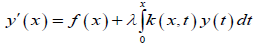
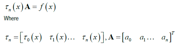
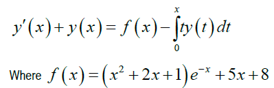
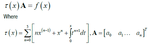
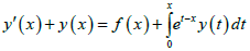
In this work, we consider Volterra Integro-differential equation of the form:

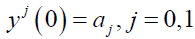
Subject to initial condition;

Where y^j = d^jy / dy^j y(x) is the unknown function, f(x) is a known function, λ is a known constant and k(x,t) is the integral kernel function.

Basic Definitions

This section defines the basic terms that will be frequently used during the research work.

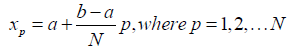
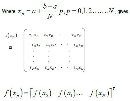
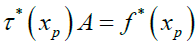
Definition 1: Standard Collocation Method: This is the method partitioning intervals into different points. For example, let say an interval [a,b], N be the number of collocation points to get the desired collocation points, we use;

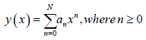
Definition 2: Power Series Polynomial: A power series is basically an infinite degree polynomial that represents some function. It is generally written in the form; Where an is the coefficient of the polynomials which are real numbers.

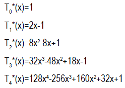
Definition 3: Shifted Chebyshev Polynomials: This is a special type of polynomial generated from Chebyshev polynomial. The shifted Chebyshev has interval [0,1], while Chebyshev has an interval of [-1,1]. The shifted Chebyshev is generated using;

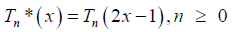
where T_n (x) is the shifted chebyshev term,while T_n (x) is the chebyshev term.

Few terms of the shifted Chebyshev terms are;

Methodology

In this section, combination of collocation method and power series approximation is employed for the numerical solution of volterra integrodfferential equations.

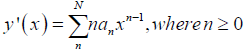
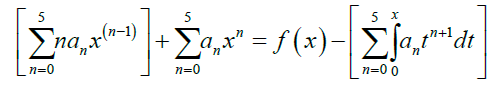
Let the solution to (1) and (2) be approximated by (3)

Where an is the real coefficients to be determined, differenting (3) with respect to x, gives

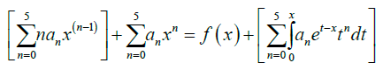
substituting (3) and (4) into (1), gives

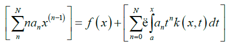
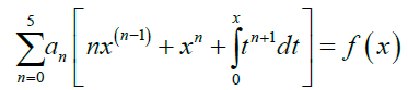
simplifying (5) gives,

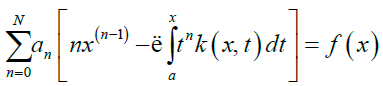
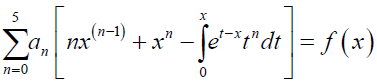
Hence,

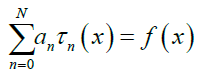
Where

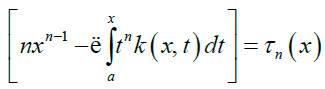
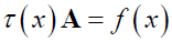
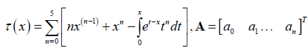
Equation (6) can be written in the form

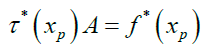
Collocating equation (7) using the standard collocation points

Considering the initial condition,

Substituting (3) into (9) we have,

Using equation(10) and equation (8) gives

Solving equation (11) using inverse multiplication to get the values of the unknown coefficient a_n, n=1, 2, …N and substituting the value of the coefficients into the approximate solution gives the numerical results. Repeating the above steps using shifted Chebyshev polynomial as the basis polynomial function, we obtained the approximate solution.

Numerical Examples: In this section, numerical examples with initial conditions are solved to confirm the efficiency and accuracy of the method. Let y_n (x) and y(x) be the approximate and exact solution respectively. Error_N = |y_n (x)-y(x)|.

Example 1: Considering Volterra integro-differential equation

subject to initial condition y(0)=10

Exact solution: y(x)=10-xe^-x

Solution 1: Solving at N = 5 using power series polynomial. Substituting approximate solution (3) into example 1 gives

Collecting the like terms gives

Equation (12) can be written in the form

collocating at 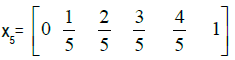and substituting the initial conditions gives

Solving equation (14), we obtained the following approximate solution

Using the above steps for solving shifted Chebyshev polynomial as the basis polynomial function, we obtained the approximate solution;

Example 2: Considering Volterra integro-differential equation

Where f(x)=0

subject to initial condition y(0)=1

Exact solution: y (x) = e^−xcosh (x)

Solution 2: Solving at N = 5 using power series polynomial. Substituting approximate solution (3) into example 2 gives

Collecting the like terms gives

Equation (15) can be written in the form

Where

collocating at 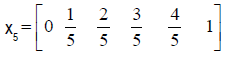and substituting the initial conditions gives

Solving equation (17), we obtained the following approximate solution (Tables 1-4).

Conclusion

The numerical solution of the Volterra integro-differential equation is presented in this study and the results are compared to the exact solution. Power series and shifted Chebyshev polynomials are used as the basis functions.

The numerical results of the examples as shown in tables shows that the results of power series approximation converges to the exact solution than the results of shifted chebyshev approximation. Observation also shows that as the value of x increases i.e. (from 0 to 1), the results of the shifted chebyshev diverges from the exact solutions.

Conflict of Interest

None.

References

1. Olumuyiwa, A. Agbolade and Timothy A. Anak. "Solution of first order Volterra linear integro-differential equations by collocation method." J Appl Math 1510267 (2017).

Google Scholar, Crossref

2. Adesanya, A. O., Yahaya Y. A., Ahmed B. and Onsachi R. O. "Numerical Solution of Linear Integral and Integro-Differential Equations Using Boubakar Collocation Method." Intern J Math Sci Optim Theory Appl 2019 (2019): 592-598.

Google Scholar

3. Gegele, O. A., Evans O. P. and Akoh D. "Numerical Solution of Higher Order Linear Fredholm–Integro–Differential Equations." Am J Eng Res 3 (2014): 243-247.

Google Scholar

4. Nemati, S., Pedro Lima and Yadollah Ordokhani. "Numerical method for the mixed Volterra-Fredholm integral equations using hybrid Legendre functions." Appl Math 2015 (2015): 184-193.

Google Scholar

5. Abubakar, A. and Taiwo O. A. "Integral collocation approximation methods for the numerical solution of high-orders linear Fredholm-Volterra integro-differential equations." J Comput Appl Math 4 (2014): 111-117.

Google Scholar

6. Ajileye, G.,. Amoo S. A. and Ogwumu O. D. "Hybrid Block Method Algorithms for Solution of first order initial value problems in ordinary differential equations." J Appl Computat Math 7 (2018): 2.

Google Scholar

7. Mehdiyeva, Galina, Mehriban Imanova and Vagif Ibrahimov. "On the Construction of the Multistep Methods to Solving the Initial-Value Problem for ODE and the Volterra Integro-Differential Equations."

Google Scholar

8. Ajileye, G., Okedayo G. T. and Aboiyar T. “Laguerre Collocation Approach for Continuous Hybrid Block Method for Solving Initial Value Problems of Second Order Ordinary Differential Equations.” Trends Food Sci Techn 2 (2017): 379- 383.

Google Scholar

9. Celik, Ercan and Khatereh Tabatabaei. "Solving a class of Volterra integral equation systems by the differential transform method." Int J Nonlinear Sci 16 (2013): 87-91.

Google Scholar

10. Uwaheren, O. A., Adebisi A. F. and Taiwo O. A. "Perturbed collocation method for solving singular multi-order fractional differential equations of Lane-Emden type." J Niger Soc Phys Sci (2020): 141-148.

Google Scholar, Crossref

11. Raftari, Behrouz. "Numerical solutions of the linear Volterra integro-differential equations: Homotopy perturbation method and finite difference method." World Appl Sci J 9 (2010).

Google Scholar

12. Bhrawy, Ali H., Emran Tohidi and Fazlollah Soleymani. "A new Bernoulli matrix method for solving high-order linear and nonlinear Fredholm integro-differential equations with piecewise intervals." Appl Math Comput 219 (2012): 482-497.

Google Scholar, Crossref

13. Fadugba, Sunday Emmanuel. "Solution of fractional order equations in the domain of the Mellin transform." J Niger Soc Phys Sci (2019): 138-142.

Google Scholar, Crossref

14. El-Kady, M. and Biomy M. "Efficient Legendre pseudospectral method for solving integral and integro-differential equations." Commun Nonlinear Sci Numer Simul 15 (2010): 1724-1739.

Google Scholar, Crossref

15. Shahooth, M. K., Ahmad R., Salman U. and Swidan W., et al. "Approximation solution of solving linear Volterra Fredholm integro differential equations of the second kind by using Berstein polynomial method." J Appl Computat Math 5 (2016): 298.

Google Scholar, Crossref