Optimizing Two Stage Production Inventory Models for Non −Deteriorating Items with a Constant Demand and Completely Backlogged

M. Dhivya Lakshmi^*
*Correspondence: M. Dhivya Lakshmi, Department of Mathematics, School of Advanced Sciences, Vellore Institute of Technology, Vellore-14, India, Email:

Keywords

Production inventory model • Backlogged • Inventory parameters • Optimum total inventory cost • Sensitivity analysis

Introduction

An inventory, indeed, is a stock of materials. Problems related to an inventory are common in manufacturing, maintenance service and business operations. Inventories may be associated with demand, production, various relevant costs. Generally, demand rate is considered to be constant, linear, quadratic, exponential, time dependent, ramp type and selling price dependent. However in present competitive market, the stock-dependent demand plays an important role in increase its demand. One of the factors in inventory system is deterioration. In an inventory system, the available storage space, budget, number of orders etc. are always limited. Hence under these constraints, classical inventory models have great importance.

With a view to solve inventory systems, it is highly essential for the business organizations to obtain the economic order quantity (EOQ) and obtaining this quantity leads to reduce the total average inventory cost. Thus, inventory control plays a vital role in running a business. So, the business organizations emphasize on inventory management and solving inventory problems. The inventory problem can only be solved if a suitable inventory model could be established which is fit for all the parameters concerned like, market demand, production rate, product’s life, etc. The innovative EOQ model is a highly demand on regular basis and when required in spite of having existence of huge number of inventory models. Inventory problems are mainly related to the proper management of the inventory which can lead to minimize the inventory cost.

Many researchers have work in the field of production inventory model to solve the real life problems by building the suitable inventory models. Initially, Harris FW [1] discussed inventory model [2]. Developed mathematical models for an inventory replenishment policy in which the units are deteriorating at a constant rate and the demand rate decreases negative exponentially [3]. derived a mathematical model for obtaining the economic order quantity for an item in which supplier permits a fixed delay in settling the amount [4]. Examined joint pricing and replenishment policy for deteriorating inventory with declining market [5]. formulated a generalized inventory model of dynamic pricing and lot-sizing by a reseller who sells a perishable good with partial backordering [6]. Discussed the effect of the backlogging rate on the economic order quantity Decision in an inventory model [7]. Presented an inventory replenishment policy for deteriorating items with shortages and partial backlogging [8]. Modeled the retailer’s inventory system as a cost minimization problem to determine the retailer’s ordering policies under trade credit financing [9]. Developed a continuous production control inventory model for deteriorating items with shortages [3]. Established the optimal inventory policies under permissible delay in payments depending on the order quantity and obtained the total minimum variable cost per unit of time [10]. Presented an economic production quantity (EPQ) model for deteriorating items with stock- dependent demand and shortages [11]. Presented an optimal solution procedure to find the optimal replenishment policy of an inventory model for non-instantaneous deteriorating items with stock-dependent consumption rate over a finite planning horizon. An EOQ model for permissible items with power demand and partial backlogging was developed by [12,13]. Discussed the production inventory model with time- varying production, time dependent demand and non-linear shortage cost under inflation and time discounting under partial backlogged [14]. Investigated the impact of an appropriate pricing and lot-sizing inventory model for a retailer in an inventory model when the supplier provides a permissible delay in payments [15]. Developed the optimal inventory policies for time-dependent deteriorating items in the presence of trade credit using the discounted cash-flows (DCF) approach [16]. Established a model for a retailer to determine its optimal price and optimal time with constant demand and constant deterioration in trade credit [17]. Developed an inventory model with stock dependent demand, Waybill distribution deterioration [18]. Formulated an economic lot.

Sizing production model for deteriorating items under two level trade credits [19]. Introduced an EOQ model for time-deteriorating items utilizing penalty cost with finite and infinite production rate [20]. Established an inventory model with three rates of production and time dependent deterioration rate for quadratic demand rate [21]. Proposed a mathematical model for optimum production inventory with deteriorating items and shortages [22]. Formulated economic production quantity inventory model based on the retailer’s stock level where deterioration goods follow two parameters Weibull distribution deterioration under stock dependent demand [23]. Developed an inventory model with three rates of production rate under stock and time dependent demand for time varying deterioration rate with shortages proposed an optimum inventory model for time dependent demand with shortages. In this paper, a production inventory model for non-deteriorating items with demand constant, shortages allowed and finite production rate has been proposed to minimize average total inventory cost. In the developed model, the production rate is considered to be proportional to the demand rate and a cycle is separated into four stages.

Notations and assumptions

In the developing production inventory model, the following notations and assumptions are considered.

Notations:

• D The demand rate

• P The production rate

• C₁ The holding cost per unit per unit time

• C₂ The shortage cost per unit per unit time

• C₃ The set up cost per production run

• I (t) The inventory level at time t

• TC The total inventory cost per cycle

• λ₁ The backlog production proposition

• λ₂ The stock production proposition

• F The fraction F (0 ≤ F ≤ 1) of the demand during the stock-out period

• G The fraction G (0 ≤ G ≤ 1) of the production during the stock level increasing period

• T₁ The time at which the shortage reaches its maximum and the production proces

• starts to clear all the backlogs

• T₃ The time at which the inventory level reaches its maximum and the production

• process stops

• T₄ The length of the production cycle time

Assumptions:

• Demand rate is constant.

• Production rate is constant and finite and the production rate is proportional to the demand rate.

• Lead time is zero.

• Replenishment is instantaneous.

• Deterioration rate is zero.

• Shortages are allowed and backlogged

Production inventory models for non-deteriorating items with shortages

Consider a production inventory model for non-deteriorating items in which demand rate D is constant, production rate, P that is proportional to the demand rate, lead time is zero and shortages are allowed and are backlogged.

At the time t = 0, the inventory level is zero. The shortage starts at t = 0 and accumulates up to the level A at time t = T₁. In the shortage, only a fraction F (0 ≤ F ≤ 1) of the demand during the stock-out period is backlogged (called active backlog) and the remaining fraction (1- F ) of the demand is dropped. The production starts at t = T₁ with production rate P = λ₁D

(λ₁ > 1, Fλ₁ > 1) and active backlog is completely cleared at t = T₂. At the starting time of the production, the stock-level is fixed at the level B. Based on a new information from the marketing manager during backlog closing period, only a fraction G (0 ≤ G ≤ 1) of the production during the stock-level increasing period is produced (called effective production) with production rate P = λ₂ Δ (λ₂ > 1, Γλ₂> 1) and the remaining fraction (1- G) of the production is dropped. The stock - level reaches at level GB at t = T₃. The production stopped at level t = T₃. Then, the inventory level decreases gradually due to demand and becomes zero at t = T₄. The cycle is completed at t = T₄ and it repels itself. Let I (t ) be the inventory level at any time t ( 0 ≤t ≤ T₄ ).

Note that the active backlog action helps us to remove all preventable backlogs and the effective production action helps us to remove avoidable production (Figure 1).

Now, the governing differential equations of the above said production inventory model with boundary conditions are given below:

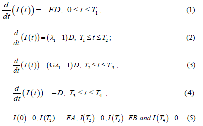
Now, solving (1) to (4) with the boundary conditions (5), we obtain the following solutions:

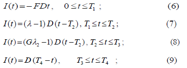
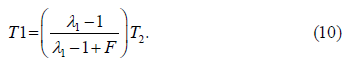
Now, using the condition I (T₁) = - FA (6) and (7), we can find that

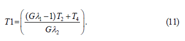
Now, using the condition I (T₃) = GB in (8) and (9), we can acquire that

Now, for finding total inventory cost, we have to find the different costs involved in the inventory system excluding the set up cost that is, total shortage cost and total inventory holding cost.

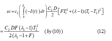
Now, the total shortage cost in the system, SC is given below:

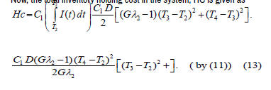
Now, the total inventory holding cost in the system, HC is given as

Now, the total inventory cost in the system, TC is given by

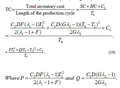
Now, we have to optimize the total inventory cost, TC which is a function T₂ and T₄.

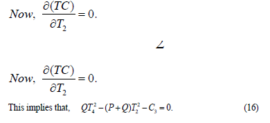
Now, solving (15) and (16), we obtain that

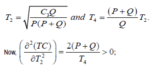
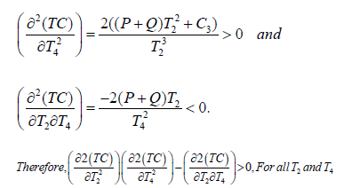
Now, the Hessian matrix for TC, H is given below:

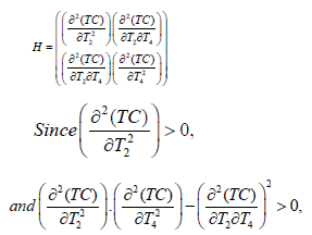
For all T₂ and T₄, H is positive definite for all T₂ and T₄

Therefore, TC is convex. This implies that the total inventory cost per cycle, TC is attained its minimum at

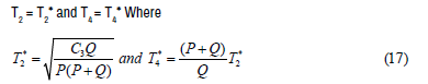
Now, from (14), (10) and (11) and using the values T₂ = T₂* and T₄ = T₄*, the optimum values of TC,T₁ and T₃ denoted by TC*,T₁ * and T₃ respectively are determined.

Numerical Example and Sensitivity Analysis : In this section, we present a numerical example to illustrate the proposed model and study the sensitivity analysis of the proposed model.

Numerical example: Consider a production inventory model for nondeteriorating items with shortages where

Now, from (17), we obtain the optimal values of T₂ and T₄ as given below:

T₂*= and 0.1070 T₄* = 1.1424.

Now, substituting the optimal values of T₂ and T₄ in (10), (11) and (14), we find the optimum values of T₁, T₃ and TC as follows

T₁ 0.0292, T₃* and 1.1074 and TC* = 70.0280.

Sensitivity Analysis: In the proposed model, there are eight parameters. They are demand (D), backlog

production proposition (λ₁), stock production proposition (λ₂), holding cost (C₁), shortage cost

(C₂), ordering cost (C₃), backlog fraction (F) and stock production fraction (G) (Table 1 and 2).

Observation

• We observe that if demand D increases and all other parameters are fixed, the optimal total inventory cost TC increases, but the optimum time values T₁, T₂, T₃ and T₄ decrease.

• It is clear to know that if the backlog production proposition λ₁ increases and all other parameters are fixed, the optimal total inventory cost TC and and the optimum time value T₁ increase, but the other optimum time values T₂, T₃ and T₄ decrease.

• We can conclude that if the stock production proposition λ₂ increases and all other parameters are fixed, the optimal total inventory cost TC and the optimum time values T₁ and T₂ increase but the other optimum time values T₃ and T₄ decrease.

• We obtain that if the holding cost C₁ increases and all other parameters are fixed, the optimal total inventory cost TC and the optimum time value T₁ increase, but the other optimum time values T₂, T₃ and T₄ decrease.

• It is clear to understand that if the shortage cost C₂ increases and all other parameters are fixed, the optimal total inventory cost TC increases but all the optimum time values T₁, T₂, T₃ and T₄ decrease.

• We observe that if the setup cost C₃ increases and all other parameters are fixed, the optimal total inventory cost TC and all the optimum time values T₁, T₂, T₃ and T₄ increase.

•We notice that if the backlog fraction F increases and all other parameters are fixed, the optimal total inventory cost TC increases, but all the optimum time values T₁, T₂, T₃ and T₄ decrease.

• We observe that if the production fraction G increases and all other parameters are fixed, the optimal total inventory cost TC and the optimum time values T₁ and T₂ increases, T₃ and T₄ decrease.

Results and Conclusion

A production inventory model for non-deteriorating items has been developed where the demand rate of a product is constant, the production rate is greater than demand rate and proportional to the demand rate, shortages are backlogged, the replenishment rate is infinite in this paper. In the proposed model, the active backlog and the effective production are considered for removing all preventable backlogs and avoidable production which are assisted to profit of the organization and a cycle has been separated into four different stages. The optimum average total inventory cost of a cycle and the optimal time for each stage for the proposed production model are determined. The developed model is illustrated with a numerical example. The considering production inventory model has been analyzed sensitively with respect to each one of its parameters.

References

1. Harris.,F.W. Operations and Costs. A.W. Shaw Company, Chicago, (1915) 48-54.
2. Hollier, R. H., and K. L. Mak. "Inventory replenishment policies for deteriorating items in a declining market." Int J Prod Res 21 (1983): 813-836.

Google Scholar, Crossref 

3. Chung, Kun Jen, Suresh Kumar Goyal and Yung-Fu Huang. "The optimal inventory policies under permissible delay in payments depending on the ordering quantity." Int J Prod Econ 95 (2005): 203-213.

Google Scholar, Crossref 

4. Wee, H.M, Wee, Hui-Ming. "Joint pricing and replenishment policy for deteriorating inventory with declining market." Int J Prod Econ 40 (1995): 163-171.

Google Scholar, Crossref 

5. Abad, Prakash L. "Optimal pricing and lot-sizing under conditions of perishability and partial backordering." Manag Sci 42 (1996): 1093-1104.

Google Scholar, Crossref 

6. Chang, Horng-Jinh, and Chung-Yuan Dye. "An EOQ model for deteriorating items with time varying demand and partial backlogging." J Oper Res Soc 50 (1999): 1176-1182.

Google Scholar, Crossref 

7. Wang, Sheng-Pen. "An inventory replenishment policy for deteriorating items with shortages and partial backlogging." Comput Oper Res 29 (2002): 2043-2051.

Google Scholar, Crossref 

8. Huang, Yung-Fu. "Optimal retailer's ordering policies in the EOQ model under trade credit financing." J Oper Res Soc 54 (2003): 1011-1015.

Google Scholar, Crossref 

9. Samanta, G. P. "A production inventory model with deteriorating items and shortages." Yugoslav J Oper Res 14 (2016).

Google Scholar, Crossref, Indexed at

10. Jain, Madhu, G. C. Sharma, and S. H. Rathore. "Economic production quantity models with shortage, price and stock-dependent demand for deteriorating items." (2007): 159-168.

Google Scholar

11. Uthayakumar, R., and K. V. Geetha. "A replenishment policy for non-instantaneous deteriorating inventory system with partial backlogging." Tamsui Oxford J Math Sci 25 (2009): 313-332.

Google Scholar

12. Rastogi, Mohit, S. R. Singh, and P. Kushwah. "An inventory model for non-instantaneous deteriorating products having price sensitive demand and partial backlogging of occurring shortages." IntJ Oper Quant.Manag 24 (2018): 59-73.

Google Scholar, Crossref

13. Valliathal, M., and R. Uthayakumar. "The production-inventory problem for ameliorating/deteriorating items with non-linear shortage cost under inflation and time discounting." Appl Math Sci 4 (2010): 289-304.

Google Scholar, Crossref

14. Tripathi, R. P. "EOQ model with time dependent demand rate and time dependent holding cost function." Int J Oper Res Soc (IJORIS) 2 (2011): 79-92.

Google Scholar, Crossref 

15. Tripathi, R. P., and Manoj Kumar. "Credit financing in economic ordering policies of time-dependent deteriorating items." IJMSS 2 (2011): 75-84.

Google Scholar, Crossref, Indexed at

16. Tripathi, Rakesh Prakash and S. S. Misra. "An optimal inventory policy for items having constant demand and constant deterioration rate with trade credit." IJISSCM 5 (2012): 89-95.

Google Scholar, Crossref 

17. BabuKrishnaraj, R., and K. Ramsey. "An inventory model with stock dependent demand, Waybill distribution deterioration." Int J Eng Res 24 (2013): 179-186.

Google Scholar

18. Muniappan Swaminathan, K. S., and P. Muniappan. "Mathematical Model for optimum production inventory deteriorating items." App Math Sci 9 (2015): 895-900.

Google Scholar, Crossref, Indexed at

19. Vijayashree, M., and R. Uthayakumar. "An EOQ model for time deteriorating items with infinite & finite production rate with shortage and complete backlogging." ORAJ 2 (2015).

 Google Scholar, Crossref 

20. Lakshmidevi, P. K., and M. Maragatham. "An inventory model with three rates of production and time dependent deterioration rate for quadratic demand rate." IJFMA 6 (2015): 99-103.

Google Scholar

21. Kaliraman, N. K., R. Raj, S. Chandra and H. Chaudhry. "An EPQ inventory model for deteriorating items with Weibull deterioration under stock dependent demand." Int J Sci Technol Res 4 (2015): 232-236.

Google Scholar

22. Sharmila, D., and R. Uthayakumar. "An inventory model with three rates of production rate under stock and time dependent demand for time varying deterioration rate with shortages." IJAEMS 2 (2016): 239643.

Google Scholar

23. Geetha, K., N. Anusheela, and A. Raja. "An optimum inventory model for time dependent demand with shortages." Int J Math 7 (2016): 99-102.

Google Scholar