One Method for the Numerical Resolution of One Type of Fractional Differential Equation of Euler-Lagrange

L. H. D. L. Raharimina^1*, G. Rasolomampiandry² and F. Randimbindrainibe^3
*Correspondence: L. H. D. L. Raharimina, Cognitive Sciences and Applications Research Laboratory (LR-SCA), Madagascar, Email:

Keywords

Numerical resolution • Fractional derivatives • Programming under Matlab

INTRODUCTION

Fractional differential equations are becoming more and more interesting in recent years for scientists. Many authors have already studied different types of problems and have formulated Euler-Lagrange equations with different boundary conditions [1-18]. An ordinary differential equation containing a composition of left and right fractional derivatives to order α, 0< α<1, with boundary conditions, is considered in our work. This type of equation is known as the fractional differential equation of Euler-Lagrange. Fractional differential equations appear in certain fields such as physics, mechanics, electrical engineering, etc... This type of equation can be solved with other methods such as the Laplace transformation or a method using the principle of least action [10,11]. An analytical method using the fixed- point theorem [6,7] also provides a solution, but this method is complicated. This is why we propose another numerical method to solve this type of fractional differential equation. We opted the programming under Matlab language to find this numerical solution.

Research Methodology

This work will be presented in four sections: in section 2, we recall the definitions which are necessary tools for the resolution of the equation that we will presented in section 3. In section 4, we propose a numerical solution, at first we search the numerical schemes for both fractional operators occurring in equation and then we determine a developed form of equation in order to establish a system of linear equations that we will transform into matrix form. In the last section, the programming under Matlab language allowing finding approximate numerical solutions graphically and the examples of numerical solution are given.

Preliminaries

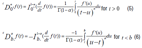
In this section, we give some useful definitions for this numerical solution. The left and right fractional integrals in the sense of Riemann-Liouville of order on an interval [0,b] are defined respectively by:

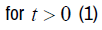
Where Γ is Euler's Gamma function and

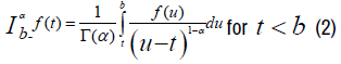
The left and right fractional derivatives of Riemann-Liouville to order α, 0<α<1 are defined from these fractional integrals to order α by:

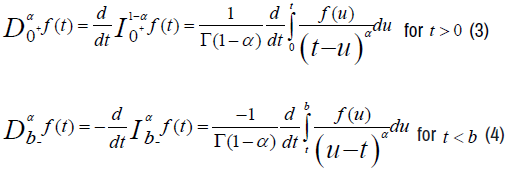
The left and right fractional derivatives to order α in the sense of Caputo are also defined from the left and right fractional integrals of Riemann-Liouville of order α by:

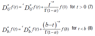
The relationship between the left fractional derivatives of Riemann-Liouville and the left fractional derivative of Caputo, both of orderα , is the following:

Presentation of the problem

We study in this work, one of type of the fractional differential equation of Euler- Lagrange of order α:

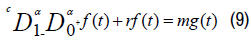
Where: f is the unknown function, g is a given function, and are respectively the left fractional derivatives of Riemann-Liouville and the right fractional derivatives of Caputo, both of order α with 0<α<1 and t∈[0,1], the boundary conditions are:

f (0)=0 and f(1)=0 (10)

Numerical resolution

To find the discrete form of equation (9), subdivide the interval [0,1] into N parts with constant step , so there exist (N + 1) points t_i, i=0,1,...., N on this interval with 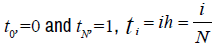are arranged in ascending order. The discrete value of the function f at each point t_i is noted f_i=f(t_i). And we note 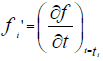the derivative of the function f at the point t_i The finite difference scheme of order 1 is written:

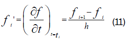
This scheme allows us to find the approximate value of the derivative of the function f_i at each point t_i.

We determine the discrete form of this equation (9) and translate the equation obtained in matrix form.

Here are the different steps to follow to find this discrete form of the equation (9).

We will present the discrete form of each type of fractional derivative, firstly the left fractional derivative of Riemann-Liouville and secondly the right fractional derivative of Caputo, of order α,0<α<1 [9,14].

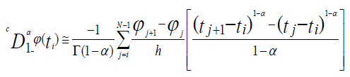
Approximation of the fractional derivative of Riemann-Liouville of order α at point t_i.

For this, we will use the relation (7) between the left fractional derivative of Riemann-Liouville and the left fractional derivative of Caputo of order α

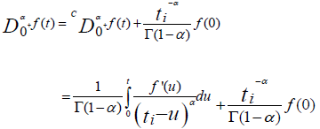
By using the approximation of the derivative by the method of finite differences (11) and by decomposing the integral, we obtain the following relation:

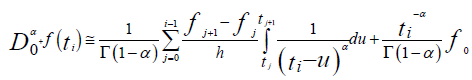
But the calculation of the integral 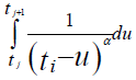gives,

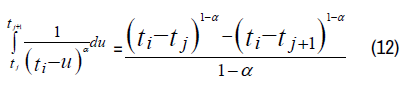
Substitute the integral by the relation (12), we get:

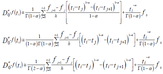
Since t_i = ih and t_j = jh then we have,

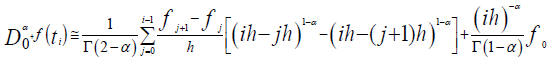
By factoring h^1-α we get the following equality:

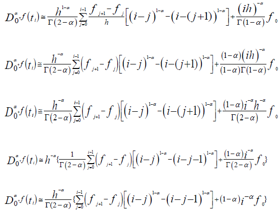
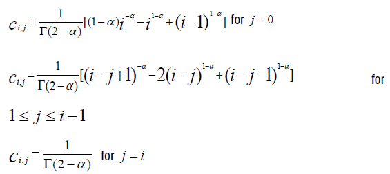
For j from 0 to i, we obtain the coefficients of f_j, noted h^-αc_i,j with:

The approximation of the right fractional derivative of Caputo of order α for the function ϕ is,

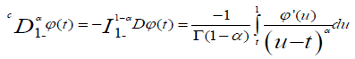
at point t_i, using the formulate of method of finite differences (11) and decomposition of the integral (12), we have:

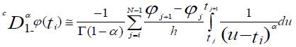
Substitute t_i and t_j by ih and jh, the approximation becomes:

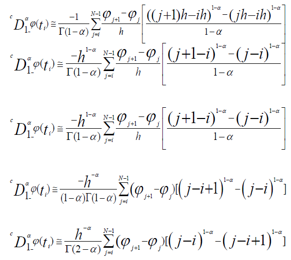
For i ≤ j ≤ N−1, we obtain the coefficients noted h^-α d_i,j of the function ϕ_j, with:

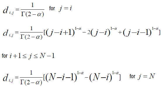
Thus, by composition of the two operators, we can write the initial equation (9) in the following discrete form:

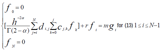
For i ranging from 1 to N-1, we get, for each value of i, the following expanded form:

Where the coefficients 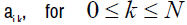, are defined by:

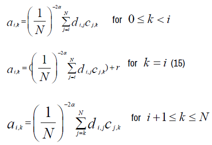
Thus, we can write the following system of N+1 equations of unknowns f_i.

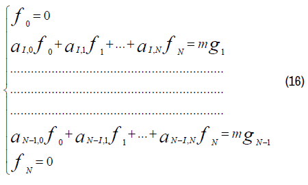
This system can be translated by matrix form:

where: (17)

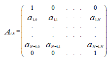, the matrix of the coefficients of f_i of the system

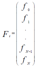the matrix of unknowns fi with i rows, 0≤i≤N

 

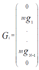the matrix equation of the second member.

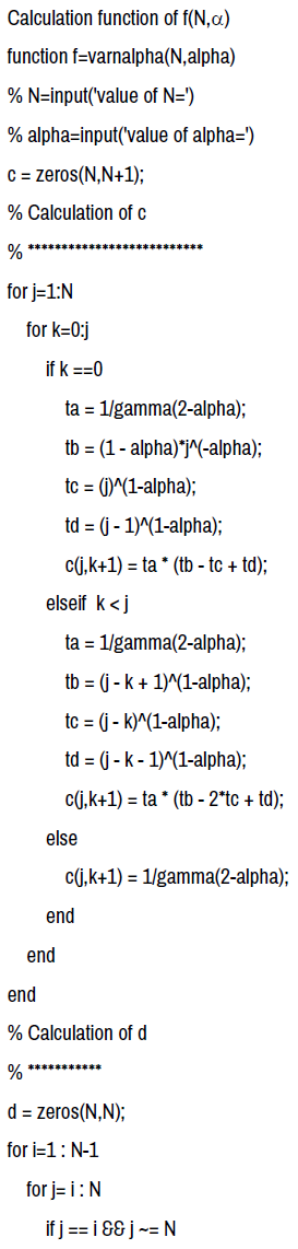
These coefficients can be calculated with programming under Matlab language that we will present below.

Programming under Matlab language and numerical examples

In this programming, firstly, we presented the case where N fixed and α varies and secondly the case where α fixed and N varies to know the influences of the values of N and those of the values of α in the results obtained graphically.

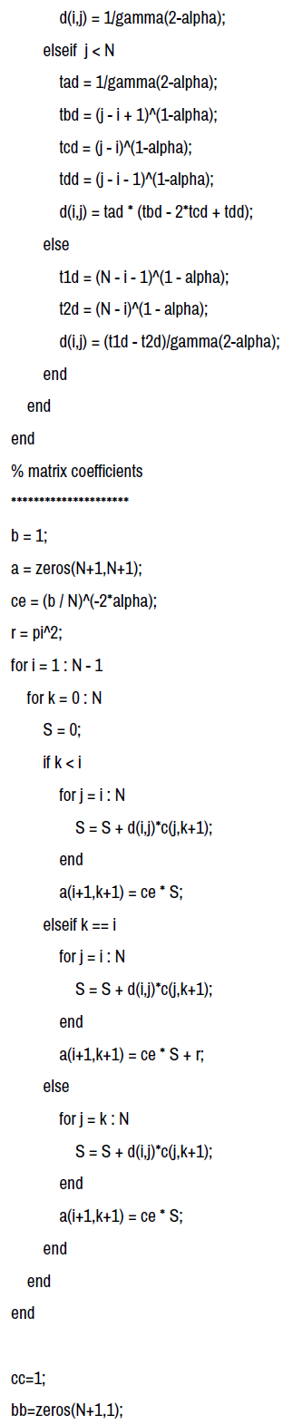
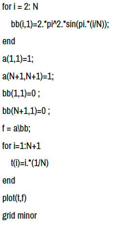
The following programming allow us to calculate step by step these coefficients c_j,k, d_i,j, a_i,k in order to represent the functions f(N,α) graphically.

In this section, the numerical results of calculations are presented. In presented solutions of equations, we assume the following parameters: for N fixed, we choose two values of N, N=100 and N=200, α ∈{0,0.1,0.2,0.8,0.9,1} but for α fixed, α = 0.1, α = 0.8, α = 0.9 , N∈{200, 300, 500, 1000}. Here, the function g, the constant r and m are given in the programming. These values of g, r and m can be changed in this programming.

In this example of programming, we take g(t) = 2π² sin(π t), r =π², m = 2π² (17).

Analyzing the graphical representations seen previously, we note that when α is fixed and N varies then the shape of all the curves are the same and they are confused for all the values of N but the maximum value of the approximate solution f_i reached is the same at the point t_i=0.5, and decreases when the value of increases. For fixed N and variable, the shape of the curves does not change and the curves are different for different values of α but the maximum values of the functions f_i as a function of t_i remain the same for different values of N. We also observe that when α is close to 0 then the curves approach the curve corresponding to α=0 and they approach the curve corresponding to α=1 when α is close to 1 (Figures 1 and 2).

Conclusion

In our work, we opted for a numerical method using programming under Matlab one of the methods allowing to find the coefficients of the matrix in order to obtain approximate solutions of the function at the point for two different cases by fixing and by varying and by fixing and by varying. Our perspective is to apply this method for different problems in certain fields such as sciences, mechanics, etc.

References

1. Kilbas, Anatoliĭ Aleksandrovich, Hari M. Srivastava and Juan J. Trujillo. “Theory and applications of fractional differential equations.” Elsevier 204 (2006): 540.

Google Scholar, Crossref

2. Dubois, F., Galucio A.C. and Point N. "Introduction to Fractional Derivation." Theory Appl Eng Tech Series (2009).

Google Scholar

3. Samko, Stefan G., Anatoly A. Kilbas and Oleg I. Marichev. "Fractional integrals and derivatives, translated from the 1987 Russian original." (1993): 1749-024.

Google Scholar

4. Baleanu, Dumitru and Juan J. Trujillo. "On exact solutions of a class of fractional Euler–Lagrange equations." Nonlinear Dynamics 52 (2008): 331-335.

Google Scholar, Crossref

5. Agrawal, Om P. "A numerical scheme and an error analysis for a class of Fractional Optimal Control problems." IDETC/CIE 49019 (2009): 1253-1260.

Google Scholar, Crossref

6. Klimek, M. "Solutions of Euler‐Lagrange equations in fractional mechanics." In AIP Conference Proceedings. American Institute of Physics 956 (2007): 73-78.

Google Scholar, Crossref

7. Agrawal, Om P. "Analytical schemes for a new class of fractional differential equations." J Phys A Math Theor 40 (2007): 5469.

Google Scholar, Crossref

8. Klimek, Małgorzata. "Fractional sequential mechanics-models with symmetric fractional derivative." Czechoslov J Phys 51 (2001): 1348-1354.

Google Scholar, Crossref

9. Goncalves, Eric. "Résolution numérique, discrétisation des EDP et EDO." Institut national polytechnique de Grenoble (2005).

Google Scholar

10. Riewe, Fred. "Nonconservative lagrangian and hamiltonian mechanics." Phys Rev E 53 (1996): 1890.

Google Scholar, Crossref

11. Riewe, Fred. "Mechanics with fractional derivatives." Phys Rev E 55 (1997): 3581.

Google Scholar, Crossref

12. Morel, J. M., Takens F. and Teissier B. "The analysis of fractional differential equations." Lecture Notes in Mathematics. Springer, Berlin (2004).

Google Scholar

13. Hilfer, Rudolf, ed. “Applications of fractional calculus in physics.” World scientific (2000).

Google Scholar

14. Yang, Qianqian, Fawang Liu, and Ian Turner. "Numerical methods for fractional partial differential equations with Riesz space fractional derivatives." Applied Mathematical Modelling 34 (2010): 200-218.

Google Scholar, Crossref

15. Robert, Janin. “Non-integer Derivatives and Integrals.” (2010).
16. Oldham, Keith and Jerome Spanier. “The fractional calculus theory and applications of differentiation and integration to arbitrary order.” Elsevier (1974).

Google Scholar

17. Błaszczyk, Tomasz. "Application of the Rayleigh-Ritz method for solving fractional oscillator equation." J Appl Math Comput Mech 8 (2009): 29-36.

Google Scholar

18. Agrawal, Om P. "Formulation of Euler–Lagrange equations for fractional variational problems." J Math Anal Appl 272 (2002): 368-379.

Google Scholar, Crossref