Research Article - (2021) Volume 0, Issue 0
Received: 26-Jun-2020
Published:
11-Jan-2021
Citation: Najam UI, Md. Rafiul Hassan and Khalid Akhtar. “Influence of Principal Component Analysis as a Data Conditioning Approach for Training Multilayer Feedforward Neural Networks with Exact Form of Levenberg-Marquardt Algorithm.” Global J Technol Optim 11 (2020): 239. doi: 10.37421/GJTO.2020.11.239
Copyright: © 2020 Qadair NU, et al. This is an open-access article distributed under the terms of the Creative Commons Attribution License, which permits unrestricted use, distribution, and reproduction in any medium, provided the original author and source are credited.
Artificial Neural Networks (ANNs) have generally been observed to learn with a relatively higher rate of convergence resulting in an improved training performance if the input variables are preprocessed before being used to train the network. The foremost objectives of data preprocessing include size reduction of the input space, smoother relationship, data normalization, noise reduction, and feature extraction. The most commonly used technique for input space reduction is Principal Component Analysis (PCA) while two of the most commonly used data normalization approaches include the min-max normalization or rescaling, and the z-score normalization also known as standardization. However, the selection of the most appropriate preprocessing method for a given dataset is not a trivial task especially if the dataset contains an unusually large number of training patterns. This study presents a first attempt of combining PCA with each of the two aforementioned normalization approaches for analyzing the network performance based on the Levenberg-Marquardt (LM) training algorithm utilizing exact formulations of both the gradient vector and the Hessian matrix. The network weights have been initialized using a linear least squares method. The training procedure has been conducted for each of the proposed modifications of the LM algorithm for four different types of datasets and the training performance in terms of the average convergence rate and a proposed performance metric has been compared with the Neural Network Toolbox in MATLAB® (R2017a).
Neural • Preprocessing • Min-max • Z-score
Real-world data in its original raw format is mostly found to be incomplete and inconsistent, lacking in certain desired behaviors or trends, and usually presents various particularities such as data range, sampling, and category. Data preprocessing is a data mining technique that involves transforming raw input data into an easily interpretable format and mostly includes data cleaning, instance selection, transformation, normalization, and feature extraction for use in database-driven applications such as customer relationship management and rule-based applications like Artificial Neural Networks (ANNs). ANN training, in particular, can be made more efficient if certain preprocessing steps are performed on the network inputs and the targets. Prior to the onset of the training procedure, it is often mathematically useful to scale the inputs and the targets within a specified range so as to render them algorithmically convenient to be processed by the network during the training procedure.
The three most commonly reported data preprocessing approaches in literature for usage in machine learning applications include the min-max normalization or rescaling, the z-score normalization or standardization, and the decimal scaling normalization; however, others such as the median normalization, mode normalization, sigmoid normalization, and tanh estimators have also been reported based on the type of ANN architecture, scope of the targeted application, and the degree of nonlinearity of the dataset selected for training the network [1-10]. The main objective of min-max normalization is to transform the original data from its current value range to a new range predetermined by the user. The most commonly employed intervals used for rescaling are (0,1) and (-1,1). Z-score normalization on the other hand transforms input data by converting the current distribution of the original raw data to a standard normal distribution with a mean of 0 and a variance equal to 1. Finally, the objective of decimal normalization is to transform the input data by moving the decimal points of values of a particular feature incorporated within the data, where the number of decimal points moved is dependent upon the maximum absolute value of the feature. A wide variety of previously reported research studies based on machine learning have exploited the aforementioned data preprocessing techniques in a number of different ways so as to render the input training data algorithmically most convenient for the ANN architecture being utilized for the training procedure. For instance, Nawi et al. [11] employed each of the aforementioned types of data preprocessing techniques in order to improve the network training efficiency as well as accuracy of four types of ANN models namely, Traditional Gradient Descent with Momentum, Gradient Descent with Line search, Gradient Descent with Gain, and Gradient Descent with Gain and Line search. The training results revealed that the use of data pre-processing techniques increased the accuracy of the ANN classifier by at least more than 95%. More recently, Nayak et al. [12] applied seven different normalization approaches on a time-series data for training two simple and two neuro-genetic hybrid network architectures for the purpose of stock market forecasting. The training process conducted on each of the selected normalization approaches resulted in a relative error of 2% for each of the sigmoid normalization and the tanh estimator techniques followed by the median normalization approach with a relative error of 4%. Similarly, Jin et al. [13] utilized the min-max as well as the normal distribution-based normalization instead of the well-known standard normal distribution-based or the z-score normalization in order to forecast Tropical Cyclone Tracks (TCTs) in the South China Sea with the help of a Pure Linear Neural Network (PLNN). Four types of datasets were collected in real-time and then mapped near to as well as far away from 0 using the two selected normalization methods. It was demonstrated that both types of normalization techniques produce similar results upon training the network on four normalized datasets as long as they map the data to similar value ranges. It was further observed that mapping the data near to 0 results in the highest rate of convergence given that sufficient number of training epochs are available to train the network. More recently, Kuźniar et al. [14] investigated the influence of two types of data preprocessing techniques on the accuracy of the ANN prediction of the natural frequencies of horizontal vibrations of load-bearing walls-data compression with the application of the principal component analysis and data scaling. It was noticed that the preprocessing accomplished by scaling of the input vectors with the full information of data without the compression produces the improvement in the Mean Squared Error (MSE) up to 91%. In a similar manner, Asteris et al. [15] predicted the compressive strength and the modulus of elasticity of sandcrete materials using a Backpropagation Neural Network (BPNN) with two hidden layers and both the min-max as well as the z-score normalization approaches for preprocessing the raw input data. Based upon the comparison of the network-predicted mechanical properties with the experimentally obtained values, it was concluded that the min-max normalization resulted in the highest values of the Pearson’s correlation coefficient amongst the previous top twenty data normalization approaches reported for the prediction of each of the aforementioned mechanical properties of sandcrete materials. In a similar fashion, Akdemir et al. [16] proposed a novel Line Based Normalization Method (LBNM) to evaluate Obstructive Sleep Apnea Syndrome (OSAS) based on real-time datasets obtained from patients clinically suspected of suffering from OSAS. Each clinical feature included in the OSAS dataset was first normalized using conventional approaches including the min-max normalization, decimal scaling, and the Z-score normalization as well as by LBNM in the range of [0,1], and then classified using the LM backpropagation algorithm as well as others including the C4.5 decision tree. As compared to a maximum classification accuracy of 95.89% evaluated using 10-fold crossvalidation for the combination of the conventional normalization approaches with C4.5 decision tree, a classification accuracy of 100% was evaluated for the combination of LBNM with C4.5 decision tree for the same validation condition. More recently, Cao et al. [17] proposed a novel Generalized Logistic (GL) algorithm and compared it with the conventional min-max and z-score normalization approaches to scale a biomedical data to an appropriate interval for diagnostic and classification modeling in clinical applications. The study concluded that the ANN models trained on the datasets scaled using the GL algorithm not only proved much more robust towards outliers in dataset classification than the other two conventional approaches, but also yielded the greatest average Area Under the Receiver Operation Characteristic Curves (AUROCs) as well as the highest average accuracies than the other two normalization strategies.
All of the aforementioned studies have utilized a variety of preprocessing techniques in order to achieve the most optimum network performance whereby the structure of the training data itself has been observed to be the most decisive factor in the selection of the most appropriate method. However, none of the training algorithms proposed by each of these studies involve exact formulations of either the gradient vector or the Hessian matrix for the purpose of weights update in the training algorithm. This study proposes a first attempt of analyzing the effects of data preprocessing on the training performance of a feedforward neural network with a single hidden layer using exact formulations of both the gradient and the Hessian derived via direct differentiation for weights update in the LM algorithm. The two most commonly reported data preprocessing approaches, namely the min-max and the z-sore normalization, have been used in conjunction with PCA for four different types of training datasets, namely the 2-spiral, the parity-7, the Hénon time-series, and the Lorenz time-series. The network training performance predicted in terms of the average convergence rate and a newly proposed performance metric with each of the four selected datasets as well as the two normalization approaches for the proposed LM algorithm has been compared with the corresponding performance evaluated using the Neural Network Toolbox (NNT) in MATLAB® (R2017a).
Weights update using the LM algorithm
The training procedure of an ANN can also be viewed as a least-squares curve-fitting problem, since the objective function to be minimized is the Mean Squared Error (MSE) between the network-computed matrix at the current training iteration and the target matrix, expressed as [18]:
 (1)
(1)
where W collectively represents the weights assigned to the connections between the network layers, T represents the (Npts ×M ) target matrix assigned to the output layer, P represents the (Npts ×M ) network-computed matrix at each training iteration, M denotes the total number of patterns in the training dataset, and M represents the size of each pattern in each of P and T.
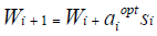
The weights update during the training process using the LM algorithm can be expressed as [18]:
 (2)
(2)
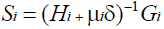
where ith represents the vector containing all the weights and biases used for the network at the ith training iteration, while αiopt and Si represent the optimal step-size and the search direction at the Si iteration respectively. For the exact form of LM algorithm, Si can be expressed as [18]:
 (3)
(3)
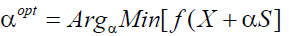
where Hi and ith represent the exact Hessian matrix and exact gradient vector at the ith training iteration, δ is the identity tensor, and μi is the learning rate at the ith iteration. For a general minimization scheme of a function f (X ) , the optimal step-size αopt can be expressed as [18]:
 (4)
(4)
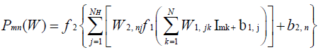
In the actual training procedure of a multilayer perceptron, the function ith in equation (4) will represent the MSE at the ith training iteration, while X will be replaced by Wi . In equation (1), a typical entry of the network-computed matrix, at a given training iteration, for a feed-forward neural network with a single hidden layer can be expressed as [18]:
 (5)
(5)
where f 1 is the activation function applied on input to each neuron in the hidden layer, f 2 is the activation function applied on input to each neuron in the output layer, I represents the (Npts× N) input matrix, I being the size of each pattern in I , NH is the number of neurons included in the hidden layer (hidden neurons), W1 represents the (NH × N) matrix consisting of weights connecting the input layer to the hidden layer, b1 represents the (NH×1) vector consisting of biases applied to each of the hidden neurons, (M ×NH) represents the (M ×NH) matrix consisting of weights connecting the hidden layer to the output layer, and (M ×1) represents the (M ×1) vector consisting of biases applied to each of the neurons in the output layer. For this study, we have selected f 1 and f 2 to be hyperbolic tangent and pure linear functions respectively, i.e., f 1 (x) = tanh(x) and f 2 (x) = x
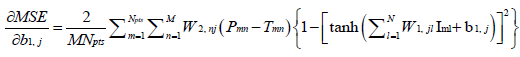
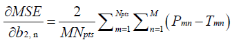
The exact gradient vector used to determine the search direction at a given training iteration in equation (3) can be expressed as [18]:
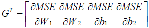 (6)
(6)
where G is a 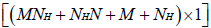 vector, and GT represents the transpose of Following substitution of equation (5) in (1), each of the first derivatives included in equation (6) can be expressed in their respective indicial notations as [18]:
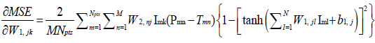 (7)
(7)
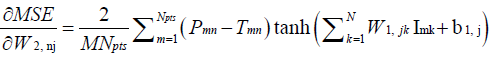 (8)
(8)
 (9)
(9)
and
 (10)
(10)
In equations (7-10), j =1,..., NH, k =1,..., N, and n =1,...,M .
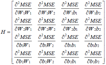
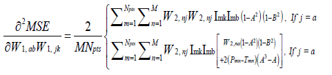
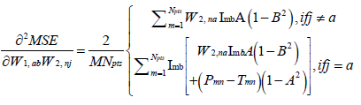
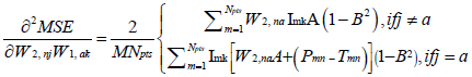
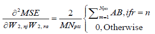
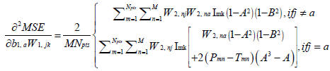
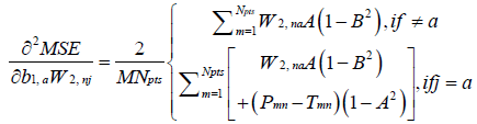
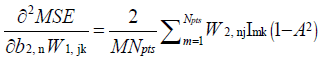
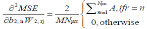
The exact Hessian matrix used to determine the search direction at a given training iteration in equation (3) can be expressed as [18]:
 (11)
(11)
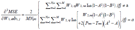
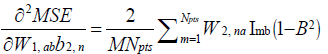
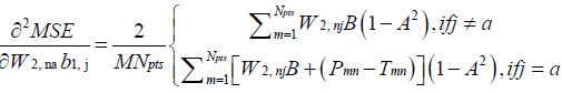
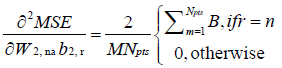
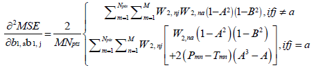
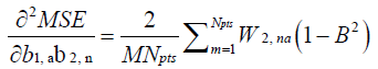
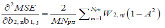
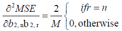
where H is a square matrix with the total number of rows or columns equal to 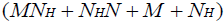 . Following substitution of equation (5) in (1), each of the second derivatives included in equation (11) can be expressed in their respective indicial notations as [18]: if j = a
 (12)
(12)
 (13)
(13)
 (14)
(14)
 (15)
(15)
 (16)
(16)
 (17)
(17)
 (18)
(18)
 (19)
(19)
 (20)
(20)
 (21)
(21)
 (22)
(22)
 (23)
(23)
 (24)
(24)
 (25)
(25)
 (26)
(26)
and
 (27)
(27)
In equations (12–27),


Weight initialization
In this work, a multilayer feedforward neural network with 3 fully interconnected layers (1 input layer, 1 hidden layer, and 1 output layer) is considered. For each of the input layer and the hidden layer, the last neuron is a bias node with a constant output equal to 1. Assuming that there are P patterns available for network training, all the given inputs to the input layer can be represented by a matrix N +1 with P rows and N+1 columns with all entries of the last column equal to 1. Similarly, the target data can be represented by a matrix T with P rows and M columns. The weights between the neurons in the input and the hidden layers form a matrix W1 with entries  , where each
  connects ith neuron of the input layer with the jth neuron of the hidden layer. Hence, the output of the hidden layer can be expressed as
  where AI ,IN ' represents the transpose of the input matrix AI ,IN ' . In a similar fashion, the weights between the neurons in the hidden and the output layers form a matrix W2 with entries
 where each W2i,j connects jth neuron of the hidden layer with the jth neuron of the output layer. This implies that the inputs to the output layer can be represented by a matrix Ao,IN with NH +1 rows and P columns. The optimal initial weights for the proposed feedforward neural network with a single hidden layer can be evaluated by solving the following minimization problem [19]:
Minimize  (28)
(28)
where W2' denotes the transpose of W2 and a typical entry of the matrix S can be expressed as:
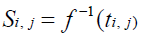 (29)
(29)
where ti, j denotes a typical entry of T. The matrix W1 is first initialized randomly following which the Linear Least Squares (LLS) problem expressed in (28) can be solved for W2OPT by QR factorization using either householder reflections or Singular Value Decomposition (SVD). However, since SVD is characterized by a relatively higther numerical stability, it has thus been utilized in the current study to solve the aforementioned minimization problem. In the case of an underdetermined system, SVD computes the minimal norm solution, whereas in the case of an overdetermined system, SVD produces a solution that is the best approximation in the least squares sense [19]. The solution W2OPT to the aforementioned LLS problem contains the optimal weights connecting the hidden layer to the output layer.
Principal Component Analysis
PCA is a statistical technique which uses an orthogonal transformation to convert a set of observations consisting of possibly correlated feature variables into a corresponding set of values of linearly uncorrelated variables commonly referred to as principal components [20,21]. The transformation is accomplished such that the first principal component accounts for the magnitude of the largest possible variability while each succeeding component sequentially characterizes continuously decreasing levels of variability within the original dataset. In the context of machine learning applications, PCA attempts to capture the major directions of variations by performing the rotation of the raw training dataset from its original space to its principal space. The magnitudes of the resulting eigenvalues thus characterize the sequentially varying levels of variability in the original dataset, while the corresponding eigenvectors which form an uncorrelated orthogonal basis define the respective directions of variation assigned to each level of variability. However, it is worth mentioning here that PCA is fairly sensitive towards the pre-scaling or normalization of the input variables included in the original dataset.
In order to conduct the PCA for an input dataset I with rows Ii, i =1,...,Npts, and columns Ij, j =1,..., N, the following stepwise procedure is followed [21]:
A new dataset S is evaluated from the original dataset I using either the min-max or z-the score normalization approaches, the typical entry of which can be expressed as:
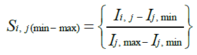 (30)
(30)
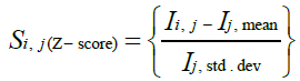 (31)
(31)
where Ij, min and Ij, max represent the minimum and maximum values in Ij respectively, while Ij, mean and Ij, std . dev represent the mean and the standard deviation of the values in Ij respectively.
The covariance matrix is then computed from the normalized dataset as:
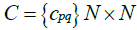 (32)
(32)
where  (33)
(33)
The eigenvectors of the covariance matrix are then determined by solving the following eigenvalue problem:
 (34)
(34)
such that 
where  is the kth eigenvalue and N represents its corresponding eigenvector. Each of the N eigenvectors determined by solving (34) are referred to as the principal components.
The eigenvalues λk are then sorted in descending order, and a matrix R is defined the columns of which are formed by the respective eigenvectors corresponding to the sorted eigenvalues.
Compute the rotation matrix R :
 (35)
(35)
where E is a diagonal matrix with diagonal entries representing the sorted eigenvalues.
The original input dataset is finally rotated using the rotation matrix to achieve a new input dataset with linearly uncorrelated patterns as:
 (36)
(36)
It is observed that all the weights used for the training procedure remain unchanged except W1 which can be recovered as:
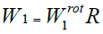 (37)
(37)
where W1 represents the W1 matrix applicable to the rotated version of the original input dataset.
Training Datasets
2-spiral dataset
The governing equations used for generating the 2-spiral dataset can be expressed as [18,22]:
where
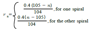

 (38)
(38)
where 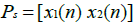 represents a typical pattern of the input matrix P,
 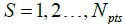 . The targeted output Ts equals 1 if the two inputs in a given pattern correspond to a point on one spiral, and -1 if they correspond to a point on the other spiral (or vice versa). Hence the total number of patterns, Npts, , contained in the dataset equals 2n . For this study, the value of n is chosen to be equal to 100 which corresponds to Npts = 200 Figure 1 shows a graphical illustration of the 2-spiral dataset.

Figure 1. Graphical illustration of the 2-spiral dataset for n = 100.
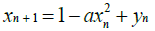
Hénon time series: The Hénon map takes a point (xn, yn) in the x-y plane and maps it to a new point [23]:
 (39)
(39)
The map depends on two parameters, a and b, which for the classical Hénon map have values of a = 1.4 and b = 0.3. For the classical values the Hénon map is chaotic. For other values of a and b the map may be chaotic, intermittent, or converge to a periodic orbit. Figure 2 shows the Hénon time series plot for the aforementioned values of a and b used in this study.

Figure 2. Hénon attractor map for a = 1.4 and b = 0.3.
Lorenz time series: The Lorenz time series is expressed mathematically by the following system of three ordinary differential equations [24]:
x = σ( y − x)
y = x(ρ − z) − y
z = xy −βz (40)
where the constants σ, ρ, and β are system parameters proportional to the Prandtl number, the Rayleigh number, and certain physical dimensions of the system respectively. For this research, the x-component of the time-series has been used as the training dataset where the values of σ, ρ, and β have been selected to be 10, 28, and 8/3 respectively for which the Lorenz time series plot is graphically illustrated in Figure 3.

Figure 3. Lorenz attractor map for σ = 10, ρ = 28 and β = 8/3.
Parity-N problems: The N -bit parity function is a mapping defined on 2N distinct binary vectors that indicates whether the sum of the N components of a binary vector is odd or even. Let 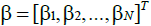 be a vector in BN where
 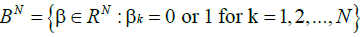 . The mapping ψ :BN → B1 is called the N -bit parity function if [18]:
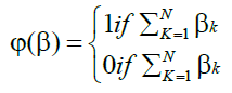 (41)
(41)
For this study, the parity-7 problem has been selected for the purpose of comparing the network performance observed using the proposed LM algorithm with that evaluated using the NNT (MATLAB® R2017a).
Training methodology: The training methodology proposed in this work using the LM algorithm with exact gradient and Hessian is demonstrated in Figure 4. The learning rate has been updated according to [18]:

Figure 4. ANN training methodology proposed in this work.
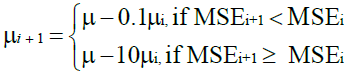 (42)
(42)
where MSEi denotes the value of MSE at the ith training iteration. For the purpose of investigating the effect of the initial value of learning rate on the training performance, two different initial values of μinit =10-1 and μinit =10-3 have been selected both of which have been updated during the training process in accordance with equation (42). The training performance of each of the proposed LM algorithm as well as the NNT (MATLAB® R2017a) has been evaluated in terms of the Average Convergence Rate (A.C.R) and a newly proposed Performance Metric (P.M) each of which can be mathematically expressed as:
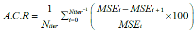 (43)
(43)
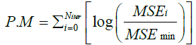 (44)
(44)
where Niter = 300 represents the selected total number of training iterations and MSE min denotes the minimum value of MSE achieved at the end of the training procedure by either of the proposed LM algorithm or the NNT (MATLAB® R2017a).
The training process using the proposed LM algorithm with direct differentiationbased exact formulations of both the gradient and the Hessian was conducted on an Intel® i7-2600 workstation with a 3.2 GHz microprocessor and 8 GB RAM. The results obtained as a result of the training process for each of the four selected datasets are discussed below.
2-spiral dataset
Figure 5 presents a comparison of the training performance of the proposed LM algorithm using either the min-max or the z-score normalization approaches with the NNT (MATLAB® R2017a) for the 2-spiral dataset. Accordingly, Table 1 presents the percentage improvement evaluated for the proposed LM algorithm over the NNT in training the network with each of the two selected preprocessing approaches for this dataset. It can be seen that the best training performance improvement for the proposed LM algorithm over the NNT has been evaluated for the case of min-max normalization as the data conditioning approach resulting in an almost 435% higher value of P.M. for NH = 2 and μinit =10-1, while the worst has been observed for the case of z-score normalization for which an almost 99% lower value of A.C.R has been obtained for NH = 2 and μinit =10-3 . Averaging the data given in Table 1 over the four selected values of NH and the two different values of μinit , the proposed LM algorithm results in an almost 81% lower value of A.C.R and a 106% higher value of P.M. than the NNT when min-max normalization is used as the data preprocessing technique, while a 91% lower value of A.C.R and a 3% higher value of P.M. for the case when z-score normalization is employed. Figure 6 demonstrates the evolution of MSE during the course of network training for each of these two scenarios of performance improvement of the proposed LM algorithm over the NNT.
| μinit | NH | Z-Score | Min-Max | ||
|---|---|---|---|---|---|
| A.C.R (%) | P.M. (%) | A.C.R (%) | P.M. (%) | ||
| 10-1 | 2 | -80.292 | 98.0884 | -50.2852 | 435.4122 |
| 5 | -90.2601 | 45.6079 | -81.7397 | 254.748 | |
| 10 | -97.5178 | -77.8631 | -83.5821 | 106.7875 | |
| 15 | -98.619 | -83.691 | -95.8307 | -56.309 | |
| 10-3 | 2 | -99.3306 | -67.9872 | -98.3184 | -13.8146 |
| 5 | -64.6449 | 272.545 | -59.0728 | 99.5533 | |
| 10 | -98.1997 | -89.2863 | -87.2132 | 89.8879 | |
| 15 | -97.0214 | -71.9453 | -94.069 | -69.6066 | |

Figure 5. Variation of average convergence rate (ACR) and proposed performance metric (P.M.) with no. of hidden neurons for the 2-spiral dataset [(a),(c): μ =10−1, (b), (d): μ =10−3].

Figure 6. Evolution of MSE during network training with the proposed LM algorithm and the NNT for the 2-spiral dataset: (a) best performance improvement (NH = 2 and μinit =10-1); (b) worst performance improvement (NH = 2 and μinit =10-3).
A careful investigation of Figure 6b reveals that the proposed LM algorithm initiates the training process with a value of MSE which is only 2% smaller than the value reached at the end of network training in contrast to the NNT for which the initial value of MSE has been observed to be 76% lower than the value achieved at the end of a premature training process consisting of only 58 epochs due to an unexpected exponential increase in the current value of μ . This clearly indicates that the most contributing factor towards the computed value of A.C.R is the magnitude of the difference between the initial and the final values of MSE in which the NNT apparently predominates owing to the incorporation of a sophisticated weight initialization procedure in the proposed LM algorithm resulting in a value of MSE as close as possible to the value achieved at the end of the training procedure. In this context, the proposed performance metric thus appears to be a more reliable performance measure than the average convergence rate since it not only encompasses the rate of decrease in the current value of MSE more efficiently with the progressive number of epochs, but also incorporates the effectiveness of the selected weight initialization approach towards the overall performance of the training algorithm. Table 2 displays the trend in the training performance improvement observed in terms of P.M. with the variation in the number of hidden neurons and the initial value of the learning rate for which the performance evaluated for NH = 2 and μinit =10-1 for each training algorithm has been referred to as the baseline reference. In case of the NNT, it can be easily noticed that the training performance not only improves with increasing μinit but also with reducing the value of μinit from 10−1 to 10−3 for each value of NH . In contrast, no such definite trend can be observed either with increasing NH or decreasing μinit for the proposed LM algorithm regardless of which of the two normalization approaches selected for data conditioning in the current study have been employed.
| Algorithm | Minit | P.M. (%) | |||
|---|---|---|---|---|---|
| NH=2 | NH=5 | NH=10 | NH=15 | ||
| NNT | 10-1 | 0 | 82↑ | 93 | 95↑ |
| 10-3 | 71↑ | 83↑ | 95 | 96↑ | |
| Min-Max | 10-3 | 0 | 72↑ | 82 | 42↑ |
| 10-3 | 81↓ | 57↑ | 86 | 25↑ | |
| Z-score | 10-1 | 0 | 75↑ | 38 | 43↑ |
| 10-3 | 80↓ | 92↑ | 9 | 70↑ | |
Hénon time series dataset
Figure 7 displays a comparison of the training performance of the proposed LM algorithm using either the min-max or the z-score normalization approaches with the NNT for the Hénon time series dataset. Accordingly, Table 3 presents the percentage improvement evaluated for the proposed LM algorithm over the NNT in training the network with this dataset using each of the two selected preprocessing approaches. It can be seen that the best training performance improvement has been evaluated for min-max normalization as the data conditioning approach which results in an almost 49% higher value of P.M. for NH = 5 and μinit, while the worst has been predicted for the case of z-score normalization which shows an almost 53% lower value of A.C.R than the NNT for NH =15 and μinit =10-1 Averaging the data given in Table 3 over the four selected values of NH and the two different values of μinit, the proposed LM algorithm results in an almost 33% lower value of A.C.R while a 15% lower value of P.M. than the NNT when min-max normalization is used as the data preprocessing technique, while a 36% lower value of A.C.R and a 16% lower value of P.M. for the case when z-score normalization is employed. Each of the two aforementioned cases of performance improvement have been demonstrated in Figure 8 in terms of the MSE evolution profiles obtained during the course of network training using the proposed LM algorithm as well as the NNT. A detailed examination of Figure 8 reveals that the training process visualized in Figure 8b conducted using the proposed LM algorithm not only initiates with a value of MSE which is almost 100% smaller than the corresponding value observed in Figure 8a, but also ends with an MSE value being almost 79% smaller. This fact coupled with the observation that the initial value of MSE observed for the training process conducted using the proposed LM algorithm in Figure 8b is 200% smaller than the corresponding value observed using the NNT, with the final value being only 56% larger, the proposed performance metric thus gauges the training efficiency of the proposed LM algorithm more accurately than the A.C.R as also observed earlier in case of the 2-spiral dataset. Table 4 displays the trend in the training performance improvement observed in terms of P.M. with the variation in the number of hidden neurons and the initial value of the learning rate where the performance evaluated for NH = 2 and μinit =10-1 for each training algorithm has been referred to as the baseline reference. It can be noticed that there is absolutely no definite trend which can be observed with either increasing NH or decreasing μinit in case of the NNT. In contrast, an increase in performance improvement can be observed for the proposed LM algorithm using the min-max normalization approach with reduction in μinit from 10−1 to 10−3 for all values of NH except for NH =15 , while a corresponding decrease can be noticed for the case of z-score normalization with the exception of NH = 5 . However, absolutely no definite trend in performance improvement with increasing NH can be observed for either of these two data conditioning approaches regardless of the initially selected value of μ as discussed above for the case of the NNT.

Figure 7. Variation of average convergence rate (ACR) and proposed performance metric (P.M.) with no. of hidden neurons for the Hénon dataset [(a),(c): μ =10−1, (b),(d): μ =10−3].

Figure 8. Evolution of MSE during network training with the proposed LM algorithm and the NNT for the Hénon time series dataset: (a) best performance improvement NH = 5 and μinit =10-3); μ = − (b) worst performance improvement ( NH = 15 and μinit =10-1).
| μinit | NH | Z-Score | Min-Max | ||
|---|---|---|---|---|---|
| A.C.R (%) | P.M. (%) | A.C.R (%) | P.M. (%) | ||
| 10-1 | 2 | -28.4616 | -27.7947 | -31.0741 | -40.0539 |
| 5 | -39.6204 | -27.4269 | -28.1732 | -9.2062 | |
| 10 | -33.3885 | -9.4681 | -45.7471 | -31.8946 | |
| 15 | -52.8348 | 10.7603 | -40.4666 | 5.6797 | |
| 10-3 | 2 | -31.8380 | -34.4650 | -33.7811 | -37.0933 |
| 5 | -10.5531 | 18.1308 | -5.7137 | 48.5464 | |
| 10 | -39.0565 | -32.7276 | -41.0382 | -27.0443 | |
| 15 | -49.4055 | -26.4054 | -38.2735 | -24.7421 | |
| Algorithm | μinit | P.M. (%) | |||
|---|---|---|---|---|---|
| NH=2 | NH=5 | NH=10 | NH=15 | ||
| NNT | 10-1 | 0 | 12↓ | 1↓ | 58↓ |
| 10-3 | 2↓ | 52↓ | 6↑ | 14↓ | |
| Min-Max | 10-1 | 0 | 26↑ | 11↑ | 11↑ |
| 10-3 | 3↑ | 39↑ | 23↑ | 9↑ | |
| Z-score | 10-1 | 0 | 11↓ | 20↑ | 3↓ |
| 10-3 | 12↓ | 7↑ | 1↓ | 12↓ | |
Lorenz time series dataset
Figure 9 displays a comparison of the training performance of the proposed LM algorithm using either the min-max or the z-score normalization approaches with the NNT for the Lorenz time series dataset, while the corresponding percentage improvement evaluated for the proposed LM algorithm over the NNT in training the network using the selected values of NH and μinit is displayed in Table 5. It can be noticed that both the best and the worst performance improvement cases can be observed for the case of min-max normalization as the data conditioning approach exhibiting an almost 1281% higher value of P.M. evaluated for NH = 2 and μinit =10-3 while an almost 84% lower value of A.C.R evaluated for NH = 2 and μinit =10-1 respectively.

Figure 9. Variation of average convergence rate (ACR) and proposed performance metric (P.M.) with no. of hidden neurons for the Lorenz time series dataset [(a,c): μ =101, (b,d): μ =10−3 ]].
Averaging the data given in Table 5 over the four selected values of NH and the two different values of μinit, , the proposed LM algorithm results in an almost 41% lower value of A.C.R and a 295% higher value of P.M. than the NNT when min-max normalization is used as the data preprocessing technique, while an 11% lower value of A.C.R and a 297% higher value of P.M. for the case when z-score normalization is employed. Since each of the two aforementioned performance improvement extremes have been observed for NH = 2, the corresponding MSE evolution profiles demonstrated in Figure 10 can thus be used as a guideline for assessing the probable effects of the initial value of the learning parameter on the training performance of each training algorithm for the Lorenz time series dataset. It can be clearly observed that despite the exact same initial values of MSE, switching the value of μinit, from 10−1 to 10−3 in the proposed LM algorithm using min-max normalization as the data preprocessing approach results in lowering the value of MSE reached at the end of network training by almost 163% compared to absolutely no such reduction observed for the training process conducted using the NNT. As shown in Table 5, the value of the performance metric evaluated for the proposed LM algorithm using the min-max normalization approach is still almost 341% larger than that evaluated for the

Figure 10. Evolution of MSE during network training with the proposed LM algorithm and the NNT for the Lorenz time series dataset: (a) best performance improvement NH = 2 and μinit =10-3 ); (b) worst performance improvement (NH = 2 and μinit =10-1) . NNT for NH = 2 and μinit =10-1 .
| μinit | NH | Z-Score | Min-Max | ||
|---|---|---|---|---|---|
| A.C.R (%) | P.M. (%) | A.C.R (%) | P.M. (%) | ||
| 10-1 | 2 | -0.2371 | 1074.8 | -83.5954 | 341.3545 |
| 5 | -32.9565 | 33.9637 | -36.2007 | 67.3175 | |
| 10 | 0.7485 | 150.3618 | -20.5572 | 277.0999 | |
| 15 | -7.8662 | 78.2490 | -30.5572 | 81.1244 | |
| 10-3 | 2 | -19.6457 | 574.8324 | -30.4296 | 1280.8 |
| 5 | -41.6891 | 78.7240 | -43.9454 | 53.2122 | |
| 10 | 3.7078 | 241.2552 | -22.4300 | 180.8576 | |
| 15 | 7.4736 | 140.2018 | -58.2703 | 79.9875 | |
This not only reflects that the value of P.M. is not as sensitive towards the change in the initial value of μ as the A.C.R, but also reveals the influence of the refinement of the initial guess towards the formulation of the proposed performance metric in contrast to the predicted value of A.C.R which is apparently related inversely to the level of sophistication of the method used for weight initialization. Table 6 displays the trend in the training performance improvement observed in terms of P.M. with the variation in the number of hidden neurons and the initial value of the learning rate where the performance evaluated for NH = 2 and μinit =10-1 for each training algorithm has been referred to as the baseline reference. It can be observed that absolutely no trend in performance improvement is noticeable for both the NNT as well as the proposed LM algorithm for the case of min-max normalization, whereas data preprocessing accomplished using the z-score normalization has been observed to result in a generally increasing trend in training performance either with increasing μinit for the same value of μinit or with reduction in μinit from 10-1 to 10−3 for the same value of NH .
| Algorithm | μinit | P.M. (%) | |||
|---|---|---|---|---|---|
| NH=2 | NH=5 | NH=10 | NH=15 | ||
| NNT | 10-1 | 0 | 96↑ | 96↑ | 98↑ |
| 10-3 | 58↑ | 97↑ | 96↑ | 96↑ | |
| Min-Max | 10-1 | 0 | 90↑ | 95↑ | 95↑ |
| 10-3 | 87↑ | 90↑ | 93↑ | 91↑ | |
| Z-score | 10-1 | 0 | 67↑ | 81↑ | 86↑ |
| 10-3 | 27↑ | 78↑ | 85↑ | 82↑ | |
Parity-7 dataset
Figure 11 displays a comparison of the training performance evaluated for the proposed LM algorithm using either the min-max or the z-score normalization approaches with the NNT for the Parity-7 dataset, whereas Table 7 presents the corresponding summary of the percentage performance improvement for the proposed LM algorithm over the NNT predicted in terms of both A.C.R as well as P.M. for different values of NH and the two selected initial values of μ. It can be noticed that the proposed LM algorithm exhibits both the best and the worst performance improvement cases in terms of the proposed performance metric for min-max normalization as the data conditioning approach, with the best being almost 6030% evaluated for NH = 10 and μinit =10-3 while the worst being almost 97% evaluated for NH = 5 and μinit =10-3. Averaging the data given in Table 7 over the four selected values of NH and the two different values ofμinit, the proposed LM algorithm results in an almost 37% lower value of A.C.R and a 975% higher value of P.M. than the NNT when min-max normalization is used as the data preprocessing technique, while a 19% lower value of A.C.R and a 756% higher value of P.M. for the case when z-score normalization is employed. A close investigation of Figure 12 which displays the MSE evolution profiles for the aforementioned best and the worst performance improvement cases reveals a completely reciprocal influence of the variation in the number of hidden neurons on the training performance evaluated for the proposed LM algorithm compared to that evaluated for the NNT. More specifically, for the same value of μinit =10-3 increasing the number of hidden neurons from 5 to 10 reduces the MSE at the end of network training by almost 200% in case of the NNT, while raises it by virtually the same magnitude in case of the proposed LM algorithm. Table 8 displays the trend in the training performance improvement observed in terms of P.M. with the variation in the number of hidden neurons and the initial value of the learning rate where the performance evaluated for μinit =10-1 and μinit =10-1 for each training algorithm has been referred to as the baseline reference. It can be observed that absolutely no trend in performance improvement with either increasing NH or reducing μinit from 10-1 to 10-3 is noticeable for each of the NNT as well as the proposed LM algorithm with min-max normalization as the data conditioning approach, whereas a clearly increasing trend with increasing NH can be observed for the case of z-score normalization for μinit =10-3. Figure 13 displays the values of the MSE reached at the end of the training procedure for the NNT as well as the proposed LM algorithm with minmax normalization as the data preprocessing approach, and 5 to 10 neurons employed in the hidden layer.

Figure 11. Variation of average convergence rate (ACR) and proposed performance metric (P.M.) with no. of hidden neurons for the Parity-7 dataset [(a,c): μ =10−1, (b,d): μ =10−3].

Figure 12. Evolution of MSE during network training with the proposed LM algorithm and the NNT for the Parity-7 dataset: (a) best performance improvement NH = 10 and μinit =10-3) , (b) worst performance improvement ( NH = 5 and μinit =10-3 ).

Figure 13. Values of MSE reached at the end of network training for the Parity-7 dataset using the proposed LM algorithm and the NNT for increasing values of NH successfully classifying the Parity-7 dataset in contrast to the NNT for which+h a minimum of 7 neurons in the hidden layer are required.
| μinit | NH | Z-Score | Min-Max | ||
|---|---|---|---|---|---|
| A.C.R (%) | P.M. (%) | A.C.R (%) | P.M. (%) | ||
| 10-1 | 2 | -9.1581 | 870.2415 | -12.1602 | 187.4554 |
| 5 | 59.2163 | -42.2796 | -42.2527 | -78.0570 | |
| 10 | -45.2078 | 313.4969 | -50.9257 | 234.5603 | |
| 15 | -72.002 | 593.5522 | -71.3155 | 702.4687 | |
| 10-3 | 2 | 76.3906 | 1264.2385 | 72.3079 | 373.3809 |
| 5 | -85.7460 | -92.4457 | -92.9680 | -97.2954 | |
| 10 | 3.7078 | 2742.2 | -22.4300 | 6030.2 | |
| 15 | -75.8734 | 394.6299 | -75.6122 | 448.9363 | |
| Algorithm | μinit | P.M. (%) | |||
|---|---|---|---|---|---|
| NH=2 | NH=5 | NH=10 | NH=15 | ||
| NNT | 10-1 | 0 | 100↑ | 100↑ | 100↑ |
| 10-3 | 16↓ | 100↑ | 97↑ | 100↑ | |
| Min-Max | 10-1 | 0 | 100↑ | 100↑ | 100↑ |
| 10-3 | 30↑ | 89↑ | 100↑ | 100↑ | |
| Z-score | 10-3 | 0 | 100↑ | 100↑ | 100↑ |
| 10-3 | 18↑ | 86↑ | 99↑ | 100↑ | |
In general, the two types of training algorithms can be observed to exhibit a roughly reciprocal trend in MSE variation with increasing NH except when either 8 or 9 neurons are employed in the hidden layer for which virtually the same value of MSE is reached at the end of the training procedure. More importantly, it is worth noticing in Figure 13 that the proposed LM algorithm with min-max normalization as the data conditioning approach requires a minimum of 6 hidden neurons for.
A modified version of the LM algorithm incorporating exact forms of the Hessian and the gradient derived via direct differentiation for training a multilayer feedforward neural network with a single hidden layer has been proposed. The weights have been initialized using a linear least squares method while the network has been trained on four types of exemplary datasets namely the 2-spiral, the Hénon time series, the Lorenz time series, and the Parity-7. Two types of conventionally employed data normalization approaches, namely the min-max normalization and the z-score normalization, have been used in conjunction with principal component analysis for preprocessing the raw input data for each type of dataset. A novel performance metric (P.M.) has been formulated which, in conjunction with the average convergence rate (A.C.R), has been employed to compare the training results achieved using the proposed LM algorithm with the corresponding ones obtained using the Neural Network Toolbox in MATLAB® (R2017a). Averaging the training results over the four selected datasets, four different number of neurons in the hidden layer, and two different initial values of the learning rate, the proposed LM algorithm has been predicted to result in a 48% lower value of A.C.R and a 340% higher value of P.M. than the Neural Network Toolbox when min-max normalization has been used as the data conditioning approach, whereas a 39% lower value of A.C.R and a 260% higher value of P.M. for the case when z-score normalization has been employed. Hence, the z-score normalization as the data preprocessing approach has been predicted to yield a roughly 21% better training performance than the min-max normalization in terms of the average convergence rate, whereas the min-max normalization has been evaluated to result in an almost 27% better training performance than the z-score normalization when the proposed performance metric has been employed as the performance measure. For network training conducted on the Parity-7 dataset, the proposed LM algorithm combined with min-max normalization as the data preprocessing approach has been evaluated to result in an almost 6030% better training performance in terms of the proposed performance metric than the Neural Network Toolbox when 10 neurons in the hidden layer and an initial value of 10-3 for the learning rate have been employed. In addition, the proposed LM algorithm with min-max normalization as the data preprocessing approach needs a minimum of 6 hidden neurons for successfully classifying the Parity-7 dataset as compared to the Neural Network Toolbox for which a minimum of 7 hidden neurons are required. A careful comparison of the training results achieved in the study using the proposed LM algorithm with those obtained using the Neural Network Toolbox suggests that the proposed performance metric can be regarded as a more reliable performance measure than the average convergence rate since it not only has been observed to assess the rate of decrease in the current value of MSE more efficiently with the progressive number of epochs, but has also been noticed to incorporate the effectiveness of the selected weight initialization approach towards the overall performance of the training algorithm. The study can prove to be a valuable addition to the current literature dedicated towards the development of increasingly sophisticated machine learning algorithms designed for high-performance commercial applications.
The authors are highly thankful to the School of Mechanical and Manufacturing Engineering, National University of Sciences and Technology, Islamabad, Pakistan, for the assistance it has provided during the theoretical development of the work, as well as for offering its up-to-date computational facilities without availing which the results presented in the study would not have been possible.
Compliance with ethical statement
Conflict of interest: The authors declare that they have no mutual conflict of interest(s) to declare.
Ethical approval: This article does not contain any studies involving human participants or animals conducted by any of the authors.
Data availability statement: The sources of each of the four types of datasets which have been utilized to obtain the results of the training procedure conducted upon the selected network architecture have been cited in the “References” section of the manuscript.
Sources of funding: The authors declare that absolutely no agencies or collaborating organizations, either academic or industrial, have been involved in providing the funds required to accomplish the current format of the manuscript.
Global Journal of Technology and Optimization received 847 citations as per Google Scholar report