A Unified Method for Solving n-Order System of Equations with m Variables

Sudarshan Kumaresan Muthuselvi^*
*Correspondence: Sudarshan Kumaresan Muthuselvi, Department of Electronics and Telecommunication, Veermata Jijabai Technological Institue (VJTI), Mumbai, India, Email:

Keywords

Generalized solutions • Systems of equations • Row echelon form • Variable isolation • High-order equations • Mathematical methods • Algebraic systems • Computational techniques.

Introduction

The solution of systems of equations has long been a cornerstone of mathematical analysis and computational applications. Several classical methods have been developed to solve linear systems of equations, each with its own strengths and limitations. Among these, the Gaussian Elimination, Gauss-Jordan, Gauss-Seidel, and Gauss- Jacobi methods, as well as the LU Decomposition method, are widely recognized for their applicability in various scenarios [1].

Classical methods for solving systems of equations

Gaussian elimination and Gauss-Jordan methods: Gaussian elimination is a systematic method for solving systems of linear equations. By transforming the system’s matrix into an upper triangular form, this method fascinates back-substitution to find the solution [2]. The Gauss-Jordan method extends this approach by reducing the matrix further to its reduced row echelon form, enabling the solution to be read directly from the transformed matrix. These methods are computationally efficient and well-suited for solving systems where the number of equations equals the number of variables (n=m) [3].

Gauss-Seidel and Gauss-Jacobi iterative methods

The Gauss-Seidel and Gauss-Jacobi methods are iterative techniques used primarily for solving large, sparse systems of linear equations. These methods start with an initial guess and iteratively refine the solution. Gauss-Seidel updates the solution sequentially using the most recent estimates, while Gauss-Jacobi updates all variables simultaneously using the values from the previous iteration [4]. These methods are advantageous for their simplicity and lower computational cost per iteration, making them suitable for large systems. However, they often require good initial guesses and may converge slowly for certain types of matrices.

LU decomposition Method

The LU Decomposition method factors a matrix A into the product of a lower triangular matrix L and an upper triangular matrix U. This decomposition allows for the system Ax=b to be solved efficiently by forward and backward substitution. LU decomposition is particularly effective for solving multiple systems with the same coefficient matrix but different right-hand sides. Its computational efficiency makes it a preferred choice for large-scale problems [5].

Limitations of classical methods for higher-order systems

Despite their effectiveness for linear systems, these classical methods often struggle with higher-order and non-linear systems of equations. Systems where the equations are of higher degrees (norder) and involve multiple variables (m) present significant challenges. The computational complexity increases exponentially, and iterative methods may fail to converge or require prohibitive amounts of computational resources [6].

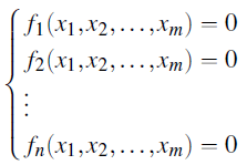
For a generalized system of equations of the form

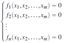
where f_i are non-linear functions, traditional methods are often insufficient. The non-linearity and potential high degree of the equations necessitate a more robust approach.

A new generalized solution method

This paper proposes a new method that extends the utility of row echelon form to solve any system of equations of order n with m variables, regardless of the system’s complexity. By iteratively treating each variable as a constant relative to the others, this method effectively reduces complex systems to a manageable series of linearlike operations. This approach not only simplifies the computational process but also provides a versatile framework capable of handling a diverse range of equation format and structures.

In the following sections, we will detail the theoretical foundation of this method, provide a step-by-step procedure for its application, and demonstrate its effectiveness through various illustrative examples.

Definitions

• Row echelon form: Row Echelon Form (REF) is a standard representation of a matrix where:
• All zero rows, if any, are at the bottom of the matrix.
• The leading entry (the leftmost non-zero entry) of each nonzero row is in a column to the right of the leading entry of the previous row.
• All entries below the leading entry of a nonzero row are zero.

Example:

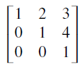
This matrix is in row echelon form because:

• The leading entry of each nonzero row is to the right of the leading entry of the previous row.
• All entries below the leading entry of each nonzero row are zero.

Literature Review

The proposed method for solving a system of non-linear equations [2] of order n with m variables involves systematically isolating each variable and leveraging row echelon form. The following steps outline the methodology in detail:

Step 1: Consider the system of non-linear equations

Given a system of non-linear equations of order n with m

variables x₁, x₂, …..., x_m

Step 2: Isolate one variable and treat others as constants

For each equation fi, isolate one variable xj and treat the remaining variables x₁,..., x_j-1, x_j+1,..., x_m as constants. Within the system, these variables take on fixed values, hence acting as constants.

Step 3: Rearrange the Equations

Rearrange each equation such that all terms involving the variable xj are on the Left-Hand Side (LHS) and all other terms, considered as constants, are on the Right-Hand Side (RHS).

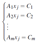
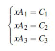
Here, A₁, A₂ ..., Am are the coefficients of xj, expressed in terms of the other variables, and C₁, C₂..., C_m are the constant terms on the RHS.

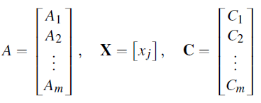
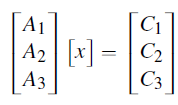
Step 4: Formulate the matrix equation

Express the system in matrix form AX=C, where

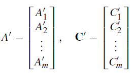
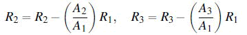
Step 5: Apply Row Echelon Form

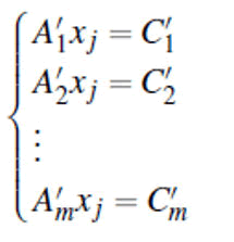
Transform the matrix equation AX=C to row echelon form, resulting in a new system A'X=C', where A' is the matrix A in row echelon form and C' is the transformed constant matrix.

Step 6: Convert back to system of equations

Convert the matrix form A'X=C' back into a system of equations.

Step 7: Expand and solve the system

Expand the coefficients A₁, A₂,...,A_m and constants C₁,C₂,...,C_m back into their original terms involving the other variables. This yields a new system of equations.

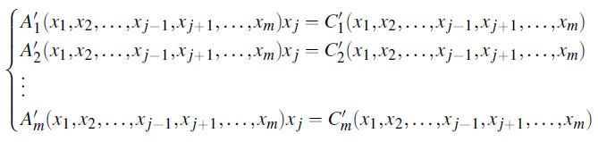
Solve this new system to find the value of x_j.

Step 8: Repeat for all variables

Repeat Steps 2 to 7 for each variable x₁, x₂,...,x_m in the original system. This process yields the solution for all variables in the system. By following these steps, the proposed method provides a systematic approach to solving systems of non-linear equations of any order n with m variables, transforming complex problems into a series of manageable linear-like operations.

Examples: Consider the following system of non-linear equations.

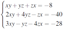
Find the values of x, y, and z.

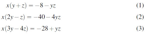
Let x be the variable and treat y and z as constants. Rearrange each equation such that terms involving x are on the Left-Hand Side (LHS) and constant terms involving y and z are on the Right-Hand Side (RHS):

Identify the coefficients A_i and constants C_i:

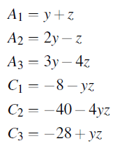
Substitute these values to obtain the new system of equations:

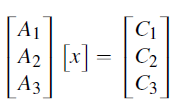
Express the system in matrix form AX=C

Apply row echelon form to the matrix A: Perform the operations.

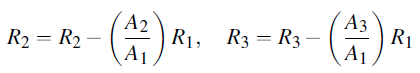
Resulting in

Transform this matrix into a set of equations:

Substitute A_i and C_i into (7), (8), (9): From equation 7:

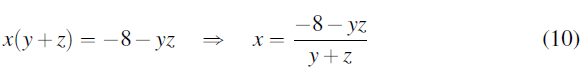
Note: y+z≠0, i.e., y≠-z.

From equation 8:

(y+z) (-40-4yz) = (2y-z) (-8-yz)

Expanding the terms:

-40y-40z-4y²z-4yz²=-16y+8z-2y²+yz²

Simplifying

-24y-32z-2y²z-3yz²=0

From equation 9:

(y+z) (-28+yz)=(3y-4z) (-8-yz)

-28y-28z+y²z+yz²=-24y+3²z-3y²z+4yz²

Simplifying:

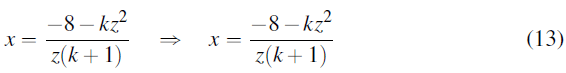
Let y=kz. Substituting this into (10), (11), (12): From Equation 10:

Note: z ≠ 0 and k ≠ -1.

From equation 11:

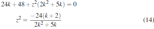
24kz+48z+2k²z³+5kz3=0

Z[(24kz+48)+z²(2k+5k)]=0

Since z ≠ 0:

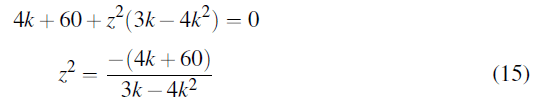
From equation 12:

4kz+60z-4k²z³+3kz3=0

z[(4k+60)+z² (3k-4k²)]=0

Since z ≠ 0:

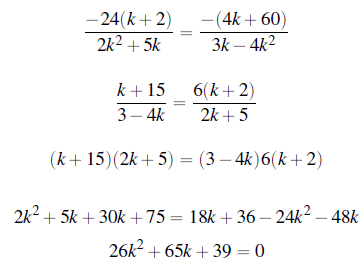
Equate (14) and (15)

on solving the quadratic equation

k=-1, k=-3/2

Since k ≠ -1

∴ k=-3/2

Since y=kz: y=3z/2

Substitute k=-3/2 into (14) or (15):

Therefore: y=3/2 × (± 2)= ± 3

Substitute y and z into (10):

x=-8-yz/y+z

For y=-3 and z=2:

x=-8-(-3 × 2)/-3+2 =-8+6/-1=2

The solutions to the system are

(x,y,z)= ± (2,-3,2)

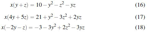
Consider the following system of non-linear equations

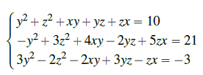
Find the values of x, y, and z

First, we let x be the variable and treat y and z as constants. Rearrange each equation such that terms involving x are on the Left- Hand Side (LHS) and constant terms involving y and z are on the Right-Hand Side (RHS).

Identify the coefficients A_i and constants C_i

A₁=y+z

A₂=4y+5z

A₃=-2y-z

C₁=10-y²-z²-yz

C₂=21+y²-3z²+2yz

C₃=-3-3y²+2z²-3yz

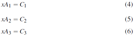
Substitute these values to obtain the new system of equations

xA₁=C₁ (19)

xA₂=C₂ (20)

xA₃= C₃ (21)

Express the system in matrix form AX=C

Apply row echelon form to the matrix A: Perform the operations:

Resulting in:

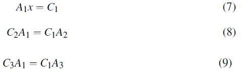
Transform this matrix into a set of equations:

A₁x=C₁ (22)

C₂A₁=C₁A₂ (23)

C₃A₁=C₁A₃ (24)

Substitute A_i and C_i

Note: y+z ≠ 0, i.e., y ≠ -z.

(y+z) (21+y²-3z²+2yz)=(4y+5z) (10-y²-z²-y²)

Expanding the terms:

21y+y³=3yz²+2zy²+21z+zy²-3z³+2yz²=40y-4y³-4zy²+50zy²-5z³-5yz²

Simplifying:

19y+29z-5y³-2z³-12zy²-8yz²=0 (26)

(y+z) (-3-3y²+2z²-3yz)=(-2y-z) (10-y²-z²-yz)

+Expanding the terms:

Simplifying: 17y+7z-5y³+z³-4yz²=0 (27)

Let y=kz. Substituting in the above equations

Where k+1 ≠ 0

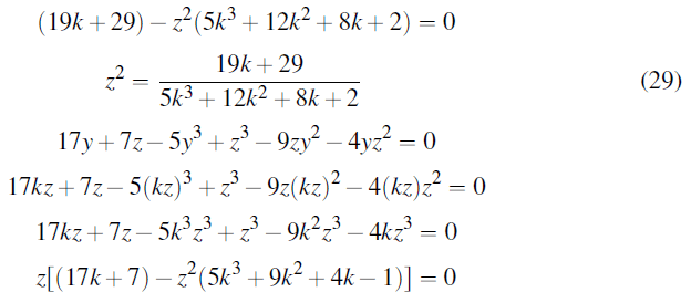
19y+29z-5y³-2z³-12zy²-8yz²=0

19(kz)+29z-5(kz)³=2z³-12z(kz)²-8(kz)z²=0

19kz+29z-5k³z³-2z³-12k²z³-8kz³=0

Z[(19k+29)-z2(5k³+12k²+8k+2)]=0

Since z ≠ 0:

Since z ≠ 0:

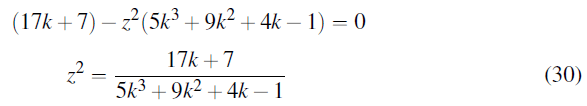
Equate equations of z²

10k⁴+77k³+117k²+7k=43

On solving for the above polynomial equation

K=-1

K=1/2

k =-5.688061...

k =-1.511938...

Since, k≠ -1

Also k =-5.688061...

and k = -1.511938...

are not definite roots.

∴k= ½

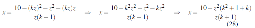
Substitute, k=1/2 in one of the z² equations

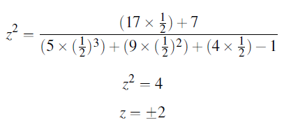
Substitute z=± 2 in y=kz,

∴y ≠ ± 1

Substituting values of y and z in equation of x, For y=1 and z=2

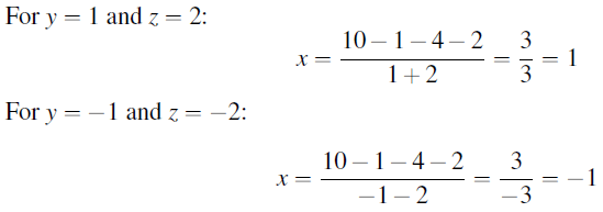
The solutions to the system are: (x,y,z)= ± (1,1,2)

Discussion

Advantages and disadvantages of the generalized method

The generalized method for solving n-order systems of equations with m variables presents several notable advantages:

Versatility: This method is highly versatile and can handle a wide variety of non-linear systems of equations. By considering one variable as the primary variable and treating the rest as constants, it simplifies the process of solving complex systems.

Standardized approach: The approach transforms the system into a standardized form, making it easier to apply matrix operations and row echelon transformations, leading to a systematic way of obtaining solutions.

Applicable to higher-order systems: Unlike traditional methods like Gauss-Jordan or LU decomposition, which are often limited to linear systems or become impractical for non-linear and higher-order equations, this method can be effectively applied to non-linear systems of any order.

Simplification through row echelon form: Utilizing row echelon form simplifies the process of isolating the main variable and reduces the system into simpler forms that are easier to solve, especially when dealing with large systems.

Despite its strengths, the method also has some limitations

• Increased iterations with more variables: As the number of variables m increases, the number of iterations required also increases. Specifically, the number of iterations needed is m-2, which can become computationally intensive for systems with a large number of variables. This can lead to a significant increase in the complexity and time required to solve the system.
• Failure condition for certain non-linear systems: Although this method is broadly applicable to non-linear systems of any order, it encounters difficulties when the n-th power of the primary variable is present in all the equations of the system. For example, consider a system of equations with variables x, y, z of order 2. If any of the equations include the term x² (assuming x is the primary variable), the method fails to provide a solution. This limitation restricts the method’s applicability in some specific cases of non-linear systems.

In the process of applying the generalized method, a special case arises when the primary variable considered at the beginning is zero. If the primary variable is zero, after transforming the matrix to row echelon form, the second and third equations obtained from the transformed matrix often result in the same equation or a multiple thereof.

This redundancy indicates that the primary variable must be zero to satisfy the system of equations. Thus, in such cases, we conclude that the value of the primary variable is zero.

Formally, if the system of equations is such that after considering the primary variable (say x), and transforming the matrix into row echelon form, the second and third equations are equivalent, this implies.

X=0

is a solution for the primary variable?

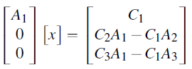
For example, consider a system of equations in the form:

After applying row echelon transformation, we get

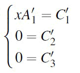
If C'₂ and C'₃ are equal or proportional, indicating a redundant equation, it implies x=0.

Therefore, we assign x=0 and proceed to solve the remaining equations for the other variables.

Conclusion

The generalized method introduced in this research provides a robust and systematic approach to solving systems of n-order equations involving m variables. This method extends beyond the capabilities of traditional techniques such as Gaussian elimination, Gauss-Seidel, and LU decomposition, which are typically confined to linear systems or become computationally impractical for non-linear and higher-order equations.

By conceptualizing one variable as the primary variable and treating the others as constants, the method effectively simplifies complex non-linear systems into more manageable forms. The utilization of matrix operations and row echelon transformations further enhances the efficiency and clarity of the solution process. This approach standardizes the manipulation of equations, making it applicable to a wide array of non-linear systems without the need for extensive customization.

Key strengths

Versatility and applicability: The method’s ability to handle systems of varying orders and degrees of non-linearity is one of its significant strengths. It provides a universal framework that can be applied to a diverse set of problems, thus offering a comprehensive solution strategy.

Systematic and structured: The step-by-step process of isolating the primary variable, transforming the system into matrix form, and applying row echelon transformations makes this method highly systematic. It reduces the potential for error and provides a clear path to obtaining solutions.

Efficient handling of higher-order systems: Traditional methods often struggle with non-linear or higher-order equations. The generalized method addresses this gap, making it suitable for solving complex systems that are otherwise challenging.

Limitations

Despite its advantages, the method is not without limitations. As the number of variables increases, the computational effort grows significantly, which may limit its practicality for very large systems. Additionally, the method encounters difficulties when the nth power of the primary variable appears in all equations, which can lead to a failure in solving the system.

Furthermore, a special consideration must be made when the primary variable is zero, as this can lead to redundant equations post row echelon transformation. In such cases, recognizing that the primary variable should be zero simplifies the solution process and ensures all potential solutions are explored.

Future Directions

Future research could focus on optimizing the algorithm for handling larger systems with multiple variables, possibly by integrating advanced computational techniques or parallel processing. Additionally, extending the method to accommodate systems where the nth power of the primary variable is present could further enhance its applicability and robustness.

In conclusion, the generalized method presents a powerful tool for solving complex systems of equations, bridging the gap left by traditional techniques and paving the way for more versatile and comprehensive solutions in mathematical and scientific computations.

References

1. Al-Kurdi, Ahmad, and David R. Kincaid. "LU-decomposition with iterative refinement for solving sparse linear systems." J Comput Appl Math 185 (2006): 391-403.

   [Crossref] [Google Scholar]

2. Boggs, Paul T. "The solution of nonlinear systems of equations by A-stable integration techniques." SIAM J Numer Anal  8 (1971): 767-785.

   [Crossref] [Google Scholar]

3. Edalatpour, Vahid, Davod Hezari, and Davod Khojasteh Salkuyeh. "A generalization of the Gauss–Seidel iteration method for solving absolute value equations." Appl Math Comput 293 (2017): 156-167.

   [Crossref] [Google Scholar]

4. Kelley, Carl T. "Solving nonlinear equations with Newton's method." SIAM J Appl Math (2003).

   [Google Scholar]

5. Khrapov, P. V., and N. S. Volkov. "Comparative analysis of Jacobi and Gauss-Seidel iterative methods." Int J Open Inf Technol 12 (2024): 23-34. [Crossref]

   [Google Scholar] [PubMed]

6. Yuster, Thomas. "The reduced row echelon form of a matrix is unique: A simple proof." Math Mag 57 (1984): 93-94.

   [Google Scholar]